As a German currently living in the US, I am amazed how completely different the discussions about the Euro crisis are inside and outside Germany. I am disappointed in the German media for completely ignoring the arguments that commentators outside Germany make. I am shocked that German economists keep conflating moral and economic issues and turn a deaf ear to sound economic advice without even engaging in a dialog. And the petty, angry and even hateful user-comments that dominate German news websites make me sad.
I would like to recommend a few articles on the current economic crisis and the Euro crisis in particular that give a much sounder picture of what is going on than can be found in the German news media at large.
Here is the gist of what I take away from all this:
I can understand the reflex to say “if you have lived beyond your means, you have to tighten your belt and save”. On the level of a single household or a single company that is sound advice. But it does not make sense at the level of an entire economy. As Paul Krugman puts it: “Your spending is my income and my spending is your income.” This means that I can only save (i.e, earn more than I spend) if there is somebody else who lives beyond his means (i.e., spends more than he earns). Therefore, it is simply impossible for everybody to save at the same time. But this is exactly what people, companies and governments all over the world are trying to do right now. People and companies try to save because of bleak economic prospects, governments try to save because they think they need to be austere. This creates a vicious cycle in which everybody tries to spend less then everybody else. The result is a depression in which nobody manages to save.
We are in a depression that is caused by a lack of demand. Therefore, propping up the supply side will not help in getting us out of this depression. So while structural reforms in the European periphery are certainly important, structural reforms alone will not get us out of this crisis, as long as demand remains depressed. And the austerity politics that Germany in particular is hell-bent on pursuing only depress demand even more.
This lack of demand creates massive unemployment (which further depresses demand). This is no accident. On the contrary, mass unemployment is the official goal of austerity politics. Austerity politics in Europe seek to achieve “internal devaluation” in the European periphery: Mass unemployment is supposed to reduce wages which in turn will restore the competitiveness of the periphery. Unfortunately, this does not work because of a phenomenon called “downward nominal wage rigidity”, which basically means that wages decrease less in a depression than they would increase in a boom. Moreover, the idea of internal devaluation disregards the catastrophic effect that mass unemployment has for the people, especially when they are young. The unemployed have to cope with huge psychological and economic pain (which even results in higher suicide rates). Also, the skills of the unemployed deteriorate which has a negative long-term effect on the economy as a whole.
An alternative means of balancing the differences in productivity between the core and the periphery is to create modest inflation in the core while keeping the inflation rate in the periphery close to zero. This would devalue the euro, making European exports more competitive on the world market. It would also create less unemployment and put less pressure on the demand in the periphery, allowing structural reforms to actually translate into economic activity.
Note that so far this has little to do with the rescue packages that seem to be the only thing that European crisis management revolves around. In fact, I think it is pointless for Germany to finance the debt of peripheral countries as long as there remains the slightest chance that peripheral governments might default. We have to make government default in Europe impossible, in exactly the same way that all other countries that are in control of their own currency do it as well: The ECB has to guarantee European sovereign debt, acting as a lender of last resort. Yes, this may amount to printing money. Yes, this will create inflation, but controlled inflation helps reducing the debt burden. Yes, this devalues the Euro, but that stimulates exports. Yes, this would amount to an implicit transfer payment from Germany to the periphery, but I am not against transfers. I am all for transfers as long as they make sense. And yes, of course this introduces a moral hazard that requires further political and financial integration to be kept in check.
German public opinion about the ever-recurring bail-out packages ranges from weary to hostile, because people rightly observe that these bail-out packages do not work but cost billions. Curiously, however, the reasons why these packages fail - from the refusal to change the ECBs role to the self-defeating mechanics of austerity - are rarely discussed in German media. Thus, most people do not realize that Merkel’s austerity is the cause of the problem. Instead, they are of the opinion that the compromises that Europeans extract from Merkel are to blame. As long as this self-serving ignorance of the German media continues, Germans will keep supporting Merkel’s policy and Merkel will keep being the hardliner that Germans expect her to be, even if Germany drops into recession.
Germans feel that they are being taken advantage of. The reasons for this lie in recent German domestic policy. The hard social security and labor market reforms that Schröder introduced with his Agenda 2010 hurt. Badly. And it took years for them to bring about economic benefits. And just now, when the sharp austerity measures that Germans themselves endured are starting to bear fruit and lead Germany into this economic boom, other countries ask Germany to step up and pay the bill for them. They didn’t do their homework and now they don’t want to endure what Germany has endured. Of course this is not entirely true, but I would claim that this is what is going on in the “German subconsciousness”. It also explains the Germans’ insistence on structural reform and their focus long-term economic outlook: these are the measures that worked for them, so these are the only measures that will work for anyone else. “There is no easy way out, so do not ask us to pay for short-term relief.”
Unfortunately, what worked for Germany in the previous decade cannot work for Europe today. There are many reasons for this. The most important one is that Germany could flourish because of its export-oriented economy. It could behave like a household that tries to earn more and spend less, because there were other countries who spent more than they earned. Now, we are in a global depression, where everybody spends too little. So the only way out is to lead Europe like an economy, not like a household. And this means stimulating demand.
Of course this will have to be at the expense of Germany. Whether this is fair or not is beside the point. It is necessary, if we do not want the world to slide into a Second Great Depression. Of course, all the unfairness entailed in and all the moral hazard created in this process will have to be addressed: No, it is not fair that the 99% pay for a crisis that the 1% caused and from which they even profited. No, it does not make sense that Germans have to work until they are 67 years old or even longer, just so that the French can enjoy an early retirement at the age of 60. And no, one country should not borrow without limit at the expense of another. But these issues can only be resolved through tighter European integration and cooperation. Trying to force tighter integration now, in the middle of this self-inflicted depression, will succeed only in fostering anti-European sentiment on all sides, without accomplishing anything.
Europe is worth paying for. And even those who do not agree should realize that this crisis will cost Germany huge amounts of money, one way or another. But when we invest these resources we have to make it count. Any workable solution needs to have widespread support in Europe. To that end we have to finally start listening to each other. We need to create a true European public and start a true dialog across national boundaries.
Recently, I have philosophized about how the mathematical community needs to move beyond (new) theorems as their currency of research. One different form of currency that I personally find particularly interesting are formal proofs. So, in the last few weeks I have spent some time getting my feet wet with one of the formal proof systems out there: HOL Light.
To learn HOL light, I decided to pick a simple theorem (from the theory of formal power series) and try to formalize it, both in a procedural and in a declarative style. In this blog post, I document what I have learned during this exercise.
My point of view is that of an everyday mathematician, who would like to use formal proof systems to produce formal proofs to go along with his everyday research papers. I realize of course, that this is not practical yet, given the current state of formal proof systems. But my goal is to get an idea of just how far away this dream is from reality.
During my experiments the hol-info mailing list was a huge help. In particular, I would like to thank Freek Wiedijk, Petros Papapanagiotou and John Harrison.
I will begin by giving a short summary of the informal proof and its two formal versions. This should give you a general idea of what all of this is about. If you want more details, you can then refer to the other parts of this post. Here is an outline:
So, without further ado, let’s start with a summary.
Summary: One Theorem and Three Proofs
The theorem that I want to prove formally is simply that every formal power series with non-zero constant term has a reciprocal - and this reciprocal has a straightforward recursive definition. In everyday, informal mathematical language, this theorem and its proof might be stated like this.
Theorem. Let $f=\sum_{n\geq 0} a_n x^n$ be a formal power series with $a_0\not = 0$. Then, the series $g=\sum_{n\geq 0} b_n x^n$ with
\begin{eqnarray*}
b_0 & = & \frac{1}{a_0} \cr
b_n & = & -\frac{1}{a_0}\sum_{k = 1}^n a_k b_{n-k} \; \forall n\geq 1
\end{eqnarray*}
is a reciprocal of $f$, i.e., $f\cdot g = 1$.
Proof. To see that $g$ is a reciprocal of $f$, we have to show that
\[
f\cdot g = \sum_{n \geq 0} \sum_{k=0}^n a_k b_{n-k} = 1
\]
which means that for all $n\in\mathbb{Z}_{\geq 0}$ we have
\[
\sum_{k=0}^n a_k b_{n-k} = \left\{ \begin{array}{ll} 1 & \text{if } n=0 \cr 0 & \text{if } n\geq 1 \end{array} \right.
\]
To show this, we proceed by induction. If $n=0$, then we have
\[
\sum_{k=0}^n a_k b_{n-k} = a_0 b_0 = a_0 \frac{1}{a_0} = 1
\]
as desired. For the induction step, let $n\in\mathbb{Z}_{\geq 0}$ and assume that the identity holds for $n$. We are now going to show that it also holds for $n+1$. To this end we calculate
\begin{eqnarray*}
\sum_{k=0}^{n+1} a_k b_{n+1-k}
& = &
a_0 b_{n+1} + \sum_{k=1}^{n+1} a_k b_{n+1-k}
\ &=&
a_0 \left( -\frac{1}{a_0}\sum_{k = 1}^{n+1} a_k b_{n+1-k} \right)
+ \sum_{k=1}^{n+1} a_k b_{n+1-k}
\ &=&
0.
\end{eqnarray*}
End of Proof.
This proof is very simple and straightforward. Therefore, many authors would try to be more terse. For example, in Wilf’s classic text book with the wonderful title generatingfunctionology this theorem is Proposition 2.1 and its proof does not even state the above calculation explicitly. Personally, I think the above proof is just about the right length.
You may have noticed that in the above proof, we did not use the induction hypothesis in the induction step. Indeed, the above proof can be done just using case analysis, without induction at all. I will nonetheless stick with the induction version of the proof, because it is more idiomatic when formalized in HOL Light.
Now, let’s see how the above proof looks when rendered in a formal proof language. In fact, we are going to do this proof in two formal proof languages: a procedural and a declarative one.
We first need to make some definitions for working with generating functions (aka formal power series). I chose to model a generating function $f$ simply as a function $f:\mathbb{N}\rightarrow\mathbb{R}$. So, if $f$ corresponds to $\sum_{n\geq 0} a_n x^n$ in the power series notation, then $f(n)=a_n$. With this approach, addition, multiplication and various other things can be defined as follows. See the section on Formal Definitions below for details.
12345
let gf_plus = new_definition `gf_plus = \(f:num->real) (g:num->real) (n:num). (f n) + (g n) :real`;;
let gf_times = new_definition `gf_times = \(f:num->real) (g:num->real) (n:num). (sum (0 .. n) (\k. (f k)*(g (n-k)))) :real`;;
let gf_one = new_definition `gf_one = \(n:num). if n = 0 then &1 else &0`;;
let gf_reciprocal = new_definition `gf_reciprocal = \(f:num->real) (g:num->real). gf_times f g = gf_one`;;
let recip = define `recip f (0:num) =  ((&1:real)/(f 0) :real) /\  recip f (n+1) = -- (&1/(f 0)) * sum (1..(n+1)) (\k. (f k) * recip f ((n + 1) - k))`;;
With these definitions, the theorem we are trying to prove is this:
1
`!(f:num->real). ~(f (0:num) = (&0:real)) ==> gf_reciprocal f (recip f)`
Note how the recursive formula for the reciprocal of $f$ has been wrapped in the definition of recip. The relation gf_reciprocal is used abbreviate the statement that recip f is a reciprocal of f.
Now we are ready to give the two formal versions of our above proof of this theorem. We start with the procedural version. It looks like this:
1234567
let GF_RECIP_EXPLICIT_FORM = prove (`!(f:num->real). ~(f (0:num) = (&0:real)) ==> gf_reciprocal f (recip f)`,
  GEN_TAC THEN DISCH_TAC THEN REWRITE_TAC[gf_reciprocal;gf_times;gf_one] THEN REWRITE_TAC[FUN_EQ_THM]
  THEN INDUCT_TAC THEN ASM_SIMP_TAC[NUMSEG_SING;SUM_SING] THEN CONV_TAC NUM_REDUCE_CONV
  THEN REWRITE_TAC[recip] THEN SIMP_TAC[REAL_ARITH `x * &1 / x = x / x`] THEN ASM_SIMP_TAC[REAL_DIV_REFL]
  THEN REWRITE_TAC[MATCH_MP (SPEC `(\k. f k * recip f (x - k))` SUM_CLAUSES_LEFT) (SPEC_ALL LE_0);SUB_0;ADD_0;ADD_AC;ADD1;recip]
  THEN (FIRST_ASSUM (ASSUME_TAC o (MATCH_MP (REAL_FIELD `!x. ~(x = &0) ==> !a. x * -- (&1 / x) * a = -- a`))))
  THEN ASM_REWRITE_TAC[] THEN SIMP_TAC[REAL_FIELD `--a + a = &0`] THEN ASM_SIMP_TAC[ARITH_RULE `~(x + 1 = 0)`]);;
I will explain this proof in detail in the section A Procedural Proof below. For now, the important thing to note here is simply this: Presented in this way, the procedural proof is completely unintelligible. To make sense of procedural proofs, they have to be run interactively. I will walk you through such an interactive run of this proof below and try to explain what is going on in the process. The gist of it is this: Procedural proofs like this one consist of a sequence of proof tactics. Tactics are essentially functions like REWRITE_TAC that are written in OCaml and that produce a part of the proof as their output. They may take pre-proved theorems like FUN_EQ_THM as their arguments.
This way of writing proofs is opposite to the way humans write informal proofs. Take for example an equational proof, i.e., a proof done by rewriting a term step by step to show an equality. Humans would write down the intermediate expressions obtained during the process. In the procedural style, you write down the rule you apply to move from one expression to the next.
While in some ways, this procedural style of carrying out a proof may in fact be closer to how humans think about proofs, this procedural notation has huge drawbacks when it comes to communicating proofs. To me, the most important drawback is that the meaning of the proof is hidden almost entirely within the library of tactics and theorems that it is built upon. Without constantly referring to a dictionary of all these ALL_CAPS_SYMBOLS it impossible to read or write these proofs at all. This is problematic insofar as it adds an additional layer of complexity to the problem of reading or writing a proof: You not only have to know the subject matter, you also have to bind yourself to a particular “API”. This not only makes proofs less human readable, it also makes procedural proofs stored in this fashion “bit-rot at an alarming rate”.
Of course, the procedural style also has its advantages, most importantly the way it lends itself to automation of proof methods. However, as I stated in the beginning, my primary concern is the translation of everyday informal mathematical articles into a formal language. Which brings us to the declarative proof style.
The declarative version of the proof that I came up with is the following:
let GF_RECIP_EXPLICIT_FORM = thm `;
  !(f:num->real). ~(f (0:num) = (&0:real)) ==> gf_reciprocal f (recip f)
  proof
    let f be num->real;
    assume ~(f 0 = &0) [1];
    !n. sum (0..n) (\k. f k * recip f (n - k)) = (if n = 0 then &1 else &0)
    proof
      sum (0..0) (\k. f k * recip f (0 - k)) = f 0 * recip f (0 - 0) by NUMSEG_SING,SUM_SING;
        .= f 0 * recip f 0;
        .= f 0 * &1 / f 0 by recip;
        .= f 0 / f 0;
        .= &1 by REAL_DIV_REFL,1;
        .= (if 0 = 0 then &1 else &0) [2];
      !n. sum (0..n) (\k. f k * recip f (n - k)) = (if n = 0 then &1 else &0)
          ==> sum (0..SUC n) (\k. f k * recip f (SUC n - k)) = (if SUC n = 0 then &1 else &0) [3]
      proof
        let n be num;
        assume sum (0..n) (\k. f k * recip f (n - k)) = (if n = 0 then &1 else &0);
        !x. ~(x = &0) ==> !a. x * -- (&1 / x) * a = -- a [4];
        sum (0..SUC n) (\k. f k * recip f (SUC n - k)) = (\k. f k * recip f (SUC n - k)) 0 + sum (0 + 1..SUC n) (\k. f k * recip f (SUC n - k)) by SUM_CLAUSES_LEFT,LE_0;
          .= (f 0 * recip f (SUC n)) + sum (1..SUC n) (\k. f k * recip f (SUC n - k)) by ADD_0,SUB_0,ADD_AC;
          .= (f 0 * recip f (n + 1)) + sum (1..(n + 1)) (\k. f k * recip f ((n + 1) - k));
          .= (f 0 * -- (&1/(f 0)) * sum (1..(n + 1)) (\k. (f k) * recip f ((n + 1) - k))) + sum (1..(n + 1)) (\k. f k * recip f ((n + 1) - k)) by recip;
          .= -- sum (1..(n + 1)) (\k. (f k) * recip f ((n + 1) - k)) + sum (1..(n + 1)) (\k. f k * recip f ((n + 1) - k)) by 1,4;
          .= &0;
          .= (if SUC n = 0 then &1 else &0);
      qed;
    qed by INDUCT_TAC from 2,3;
    (\n. sum (0..n) (\k. f k * recip f (n - k))) = (\n. (if n = 0 then &1 else &0)) [5] by FUN_EQ_THM;
  qed by gf_reciprocal,gf_times,gf_one,1 from 5;
`;;
To my eye, this looks wonderful! This is an entirely formal proof, that
is very close to the informal version,
is not that much longer than the informal version,
is human readable,
uses very few references to an external “dictionary” or “API” (not all steps have to be justified!),
and all external references refer to theorems and not to tactics.
On top of that, I had a much, much easier time writing this proof than writing the procedural version.
Of course there are still many aspects that can be improved. First of all, while this ASCII syntax is quite readable (much more readable than LaTeX anyway), the ability to edit a fully typeset version of the proof would be a pleasant convenience. I will definitely look into creating a custom transformer for Qute for this syntax.
More importantly, some steps in this proof seem unnecessarily small. For example, when calculating sum (0..0) (\k. f k * recip f (0 - k)), it would be great to go directly to f 0 * recip f 0 without using f 0 * recip f (0 - 0) as a stepping stone. In a similar vein, I would like to avoid stating trivial lemmas like !x. ~(x = &0) ==> !a. x * -- (&1 / x) * a = -- a explicitly, since in the line where it is used, it is easy to infer from context what lemma is needed here. Finally, I think it is very important to reduce API dependencies even further and so I would like to drop explicit references to such “trivial” library theorems as ADD_0 or ADD_AC.
More details about the declarative proof system and the construction of this proof make up the last part of this post.
On the whole, I am extremely impressed with the state of current formal proof systems. While a lot remains to be done until everyday mathematicians not specialized in formal proof can routinely produce formal versions of their papers, this dream appears to be almost within reach.
After this summary, I am now going to get my hands dirty and explain all of this in detail.
Meeting HOL Light
The proof system I used for these experiments is HOL Light. HOL stands for “higher order logic” which basically means classical mathematical logic with the additional feature that quantifiers can range over functions as well and not only over elements of the ground set. (In practice, working with formal higher order logic is not too different from the mix of “colloquial” classical logic and set theory that I, as a mathematician not specialized in logic, am used to working with.) Higher order logic is one of the standard foundations of mathematics used in the formal proof community and several major proof systems such as Isabelle/HOL, HOL4, ProofPower and HOL Light work with it.
In this post, I will not assume familiarity with HOL Light and I hope to keep things reasonably self-contained. Nonetheless, I want to recommend some references as starting points for further reading: Freek Wiedijk has done some very helpful work comparing and contrasting the different provers out there, see for example the list of the Seventeen Provers of the World which he compiled. To get started with HOL Light, I recommend the great HOL Light Tutorial by John Harrison. When doing a proof, it is useful to have the quick reference at hand.
Installing HOL Light is non-trivial. First, you need to have a working installation of OCaml. Second, you will need Camlp5, which has to be compiled with the -strict configuration option. This is often not the case for camlp5 packages that ship with major Linux distributions. Third, you need to fetch HOL Light from its SVN repository and compile it. I will not walk through these steps in detail, but I can recommend a script by Alexander Krauss that does these things for you (and that you can read if you need instructions on how to do this by hand).
After everything is installed, you run OCaml from the HOL Light source directory and then, from the OCaml toplevel, start HOL Light with the command
1
#use "hol.ml";;
HOL Light will need about a minute to start and will generate lots of output in the process.
In the rest of this section, I will give a very short summary of the basics of HOL Light. As an introduction to HOL Light, this whirlwind tour is of course woefully inadequate. It is mainly intended as a brief orientation for readers unfamiliar with HOL who do not want to read the tutorial first. Either way, I hope that these brief notes will help in making sense of the exercise that this post is about.
Proofs in HOL Light are typically developed interactively at the OCaml toplevel.
In HOL Light, mathematical expressions in higher order logic are enclosed in backquotes. These expressions have the OCaml type term. For example, if you enter `1 + 1 = 2` at the OCaml toplevel (followed by two semicolons and return) you will see:
12
# `1 + 1 = 2`;;
val it : term = `1 + 1 = 2`
The HOL Light syntax for higher order logic is straightforward. For example the principle of induction on the natural numbers
\[
\forall P: P(0) \wedge \left( \forall n: P(n) \Rightarrow P(S(n)) \right) \Rightarrow (\forall n. P(n))
\]
would be written as
1
!P. P 0 /\ (!n. P n ==> P (SUC n)) ==> (!n. P n)
where SUC is a predefined constant, $\forall$ is written as ! and $\wedge$ is written as /\. Here is the notation for some other useful symbols: $\exists$ is written as ?, $\vee$ is written as \/, $\neg$ is written as ~ and $\Leftrightarrow$ is written as <=>. Lambda expressions are written using \, e.g., $\lambda x. x + 1$ is written as \x. x + 1.
Higher order logic in HOL Light is typed. As long as HOL Light can figure out the types on its own, you don’t need to specify them. If you want to give type information explicitly, you can use the colon. For example, here is the principle of induction on lists:
1
!P:(A)list->bool. P [] /\ (!h t. P t ==> P (CONS h t)) ==> !l. P l
Theorems in HOL Light are objects of type thm. The only way to produce an object of type theorem in HOL Light is to prove that theorem.
Inference rules are special OCaml functions that produce theorems. They encapsulate proof methods. For example ARITH_RULE is a function of type term->thm that uses linear arithmetic methods to prove statements about natural numbers. For example we can produce the theorem $\vdash 1 + 1 = 2$ by
12
# ARITH_RULE `1 + 1 = 2`;;
val it : thm = |- 1 + 1 = 2
or we can produce the theorem $x > 0 \vdash x \geq 1$ by
12
# UNDISCH (ARITH_RULE `x > 0 ==> x >= 1`);;
val it : thm = x > 0 |- x >= 1
where UNDISCH takes a theorem of the form $\vdash p \Rightarrow q$ and produces the theorem $p \vdash q$.
A goal captures a claim of the form $p_1,\ldots,p_n\vdash q$ that we are currently trying to prove but have not proved yet. In the HOL Light documentation, the distinction is made clear using the ?- notation, e.g., the goal that $x > 0 \vdash x \geq 1$ might be written as x > 0 ?- x >= 1. On the OCaml toplevel (a stack of goals containing) this goal would be printed as:
12345
val it : goalstack = 1 subgoal (1 total)

  0 [`x > 0`]

`x >= 1`
where the expression in square brackets represents the assumption of that goal.
A tactic is a function that (essentially) takes a goal and produces a list of subgoals, such that a proof of all subgoals produces a proof of the original goal. This allows backward proofs. These are the typical way of working with HOL Light.
An example. Suppose we want to prove $x\not=0 \Rightarrow 1 \leq x$ using the lemma $0 < x \Rightarrow 1 \leq x$. We store the lemma in an OCaml variable.
12
# let lemma = ARITH_RULE `0 < x ==> 1 <= x`;;
val lemma : thm = |- 0 < x ==> 1 <= x
Then we set up our goal with the function g.
12345
# g `~(x=0) ==> 1 <= x`;;
Warning: Free variables in goal: x
val it : goalstack = 1 subgoal (1 total)

`~(x = 0) ==> 1 <= x`
Next we apply the tactic DISCH_TAC using the function e. This reduces the goal $\vdash x\not=0 \Rightarrow 1 \leq x$ to $x\not=0 \vdash 0 \Rightarrow 1$.
123456
# e DISCH_TAC;;
val it : goalstack = 1 subgoal (1 total)

  0 [`~(x = 0)`]

`1 <= x`
Now we apply our lemma to “simplify” the conclusion of our goal, using MATCH_MP_TAC which is of type thm->tactic. MATCH_MP_TAC uses the theorem $\vdash p \Rightarrow q$ to reduce the goal $\vdash q$ to $\vdash p$, making instantiations as necessary.
123456
# e(MATCH_MP_TAC(lemma));;
val it : goalstack = 1 subgoal (1 total)

  0 [`~(x = 0)`]

`0 < x`
What is now left to prove is the content of the theorem LT_NZ in the library.
12
# LT_NZ;;
val it : thm = |- !n. 0 < n <=> ~(n = 0)
We make use of this theorem via ASM_REWRITE_TAC of type thm list -> tactic, which rewrites goals by the list of (equational) theorems it is passed, taking assumptions into account.
12
# e(ASM_REWRITE_TAC[LT_NZ]);;
val it : goalstack = No subgoals
The statement that there are no subgoal left, means that the proof is complete. We can get the theorem we just proved using top_thm.
12
# top_thm();;
val it : thm = |- ~(x = 0) ==> 1 <= x
(Note that this example is non-sensical insofar as we could have used ARITH_RULE to solve our goal immediately.)
If you make a mistake during one of these goalstack-style proofs, you can use b to back up one step, by calling b();;.
After this minimal introduction to HOL Light, we can now turn to formalizing the above proof.
Formal Definitions
Before we can start with the proof proper, however, we need to make a couple of definitions.
For the purposes of this exercise a formal power series or generating function will be simply a map $f:\mathbb{N}\rar\mathbb{R}$. Of course you could also view $f$ as a sequence of real numbers or, classically, as the sequence of coefficients of a power series. Addition of formal power series is defined componentwise, i.e., $(f+g)(n)=f(n)+g(n)$, which in HOL Light looks as follows:
This simply means that gf_plus is a function that takes two generating functions and returns the generating function that is the componentwise sum of the arguments.
The product of two generating functions is defined via the Cauchy product rule
\[
(f\cdot g)(n) = \sum_{k=0}^n f(k)\cdot g(n-k).
\]
This looks much more natural when phrased in terms of formal series and this is the reason why formal power series are traditionally written in power series notation:
\[
\sum_{n\geq 0}a_nx^n \cdot \sum_{n\geq 0} b_n x^n = \sum_{n\geq0} \left(\sum_{k=0}^n a_k b_{n-k}\right) x^n.
\]
Personally, I think of this “product” more as a “Minkowski sum”, but that will be the subject of another blog post. The HOL Light version of this definition is straightforward:
Next, we define a constant gf_one which represents the formal power series $1$, i.e., the function $f$ with $f(0)=1$ and $f(n)=0$ for all other $n$.
1
let gf_one = new_definition `gf_one = \(n:num). if n = 0 then &1 else &0`;;
Now, it is straightforward to define a binary relation gf_reciprocal that specifies when a generating function $g$ is the reciprocal of a generating function $f$, that is, $f\cdot g = 1$.
1
let gf_reciprocal = new_definition `gf_reciprocal = \(f:num->real) (g:num->real). gf_times f g = gf_one`;;
Finally, the theorem we will prove contains a recursive formula for the reciprocal of a generating function $f$, namely:
\begin{eqnarray*}
b_0 & = & \frac{1}{a_0} \cr
b_n & = & -\frac{1}{a_0}\sum_{k = 1}^n a_k b_{n-k} \; \forall n\geq 1
\end{eqnarray*}
We will use the shorthand recip f to denote the function defined by this recursive formula.
1
let recip = define `recip f (0:num) = ((&1:real)/(f 0) :real) /\ recip f (n+1) = -- (&1/(f 0)) * sum (1..(n+1)) (\k. (f k) * recip f ((n + 1) - k))`;;
Note that these definitions all return theorems. In addition they have the side effect of modifying the OCaml variable the_definitions, see fusion.ml. This has the drawback that you cannot change existing definitions within a running HOL Light session. You will have to restart HOL Light to change definitions. (If you want to learn more about definitions and state in HOL, you may want to look at thesepapers.)
A Procedural Proof
The theorem that we want to prove says that if $f(0)\not= 0$ then $\text{recip}(f)$, as defined in the previous section, is a reciprocal of $f$. In HOL this statement reads simply as follows.
1
!(f:num->real). ~(f (0:num) = (&0:real)) ==> gf_reciprocal f (recip f)
Note that 0 refers to the natural number $0$, whereas &0 refers to the real number $0$ - which are distinct in HOL. Real number literals always have to be prefixed with & in HOL. The type annotations given above are not essential. We could also write simply !f. ~(f 0 = &0) ==> gf_reciprocal f (recip f).
In this section, we will go through the procedural proof given in the summary at the beginning step by step, and take a look at the goalstack at each point. If you want to expand other proofs in a similar fashion, you may want to take a look at the tool Tactician.
We start out by pushing the theorem we want to prove onto the goalstack.
1234
# g `!(f:num->real). ~(f (0:num) = (&0:real)) ==> gf_reciprocal f (recip f)`;;
val it : goalstack = 1 subgoal (1 total)

`!f. ~(f 0 = &0) ==> gf_reciprocal f (recip f)`
Next, we eliminate the universal quantifier and the implication, turning $f(0) \not = 0$ into an assumption, and we expand the definitions.
12345678910111213141516171819202122
# e(GEN_TAC);;

val it : goalstack = 1 subgoal (1 total)

`~(f 0 = &0) ==> gf_reciprocal f (recip f)`

# e(DISCH_TAC);;

val it : goalstack = 1 subgoal (1 total)

  0 [`~(f 0 = &0)`]

`gf_reciprocal f (recip f)`

#  e(REWRITE_TAC[gf_reciprocal;gf_times;gf_one]);;

val it : goalstack = 1 subgoal (1 total)

  0 [`~(f 0 = &0)`]

`(\n. sum (0..n) (\k. f k * recip f (n - k))) =
 (\n. if n = 0 then &1 else &0)`
We have to show that two functions are equal. This boils down to showing that their values are equal for all arguments. This is the content of FUN_EQ_THM, which we apply using REWRITE_TAC.
1234567
# e(REWRITE_TAC[FUN_EQ_THM]);;

val it : goalstack = 1 subgoal (1 total)

  0 [`~(f 0 = &0)`]

`!x. sum (0..x) (\k. f k * recip f (x - k)) = (if x = 0 then &1 else &0)`
Now we start working at the heart of the problem. Just as in the informal proof, we are going to use induction, even though a more elementary case analysis would work as well. To use induction we apply INDUCT_TAC which leaves us with two subgoals: The base of the induction and the induction step.
12345678910111213
# e(INDUCT_TAC);;

val it : goalstack = 2 subgoals (2 total)

  0 [`~(f 0 = &0)`]
  1 [`sum (0..x) (\k. f k * recip f (x - k)) = (if x = 0 then &1 else &0)`]

`sum (0..SUC x) (\k. f k * recip f (SUC x - k)) =
 (if SUC x = 0 then &1 else &0)`

  0 [`~(f 0 = &0)`]

`sum (0..0) (\k. f k * recip f (0 - k)) = (if 0 = 0 then &1 else &0)`
We start working on the base of the induction, i.e., the second subgoal. All we simplify the equality we have to prove, by evaluating the if .. then .. else .. and using the fact that the sum over an interval that contains just $0$ can be obtained by evaluating the expression we sum over at $0$. This latter fact follows from the lemmas NUMSEG_SING and SUM_SING.
123456
# e(ASM_SIMP_TAC[NUMSEG_SING;SUM_SING]);;
val it : goalstack = 1 subgoal (2 total)

  0 [`~(f 0 = &0)`]

`f 0 * recip f (0 - 0) = &1`
The next couple of steps are about calculating with numbers and we use a couple of different methods for doing so. NUM_REDUCE_CONV is a so-called conversion, that can be used to simplify expressions as part of a bigger expression, and conversions can be turned into tactics using CONV_TAC. NUM_REDUCE_CONV evaluates expressions over natural numbers and this allows us to reduce $0-0$ to $0$, without knowing the name of a lemma in the HOL library that says so. Afterward, we expand recip according to its definition.
1234567891011121314
# e(CONV_TAC NUM_REDUCE_CONV);;
val it : goalstack = 1 subgoal (2 total)

  0 [`~(f 0 = &0)`]

`f 0 * recip f 0 = &1`

# e(REWRITE_TAC[recip]);;

val it : goalstack = 1 subgoal (2 total)

  0 [`~(f 0 = &0)`]

`f 0 * &1 / f 0 = &1`
Next, we want to go from $f(0)\cdot \frac{1}{f(0)}$ to $\frac{f(0)}{f(0)}$. Again we don’t know the exact name of a lemma in the library that allows us to get there. However, the library does contain a general purpose inference rule REAL_ARTIH that can prove certain identities of real numbers automatically. We use this to prove the lemma we need on the fly. After this, all that is left to show is that $\frac{f(0)}{f(0)}=1$ under the assumption that $f(0)\not=0$. The appropriate lemma in the library is REAL_DIV_REFL. To apply it, we use ASM_SIMP_TAC which uses not only the theorem it is passed as argument, but also takes into account the available assumptions. This, then, completes our proof of the base of the induction, and we continue to the next goal on the stack: the induction step.
123456789101112131415
# e(SIMP_TAC[REAL_ARITH `x * &1 / x = x / x`]);;
val it : goalstack = 1 subgoal (2 total)

  0 [`~(f 0 = &0)`]

`f 0 / f 0 = &1`

# e(ASM_SIMP_TAC[REAL_DIV_REFL]);;
val it : goalstack = 1 subgoal (1 total)

  0 [`~(f 0 = &0)`]
  1 [`sum (0..x) (\k. f k * recip f (x - k)) = (if x = 0 then &1 else &0)`]

`sum (0..SUC x) (\k. f k * recip f (SUC x - k)) =
 (if SUC x = 0 then &1 else &0)`
The first thing that we want to do here is to split off the first summand of the sum. The theorem in the library that says we can split off the first term in a sum is SUM_CLAUSES_LEFT.
12
# SUM_CLAUSES_LEFT;;
val it : thm = |- !f m n. m <= n ==> sum (m..n) f = f m + sum (m + 1..n) f
We want to use this theorem for $f=\lambda k. f(k)\cdot \text{recip}(f,x-k)$, $m=0$ and $n=n$. We can achieve these specializations as follows. Here LE_0 is the theorem $\forall n. 0 \leq n$ and SPEC_ALL LE_0 is simply the theorem $0 \leq n$. Note that $n$ refers to a natural number here.
123456789101112
# let sum_lemma = (SPEC `(\k. f k * recip f (x - k))` SUM_CLAUSES_LEFT);;
val sum_lemma : thm =
  |- !m n.
         m <= n
         ==> sum (m..n) (\k. f k * recip f (x - k)) =
             (\k. f k * recip f (x - k)) m +
             sum (m + 1..n) (\k. f k * recip f (x - k))
# let split_sum_lemma = MATCH_MP sum_lemma (SPEC_ALL LE_0);;
val split_sum_lemma : thm =
  |- sum (0..n) (\k. f k * recip f (x - k)) =
     (\k. f k * recip f (x - k)) 0 +
     sum (0 + 1..n) (\k. f k * recip f (x - k))
We use our split_sum_lemma to split the sum in question. After some simplifications, the first occurrence of $\text{recip}$ in the expression is in the exact form we need in order to be able to apply the recursive definition of $\text{recip}$.
1234567891011121314151617181920212223242526272829
# e(REWRITE_TAC[split_sum_lemma]);;
val it : goalstack = 1 subgoal (1 total)

  0 [`~(f 0 = &0)`]
  1 [`sum (0..x) (\k. f k * recip f (x - k)) = (if x = 0 then &1 else &0)`]

`f 0 * recip f (SUC x - 0) +
 sum (0 + 1..SUC x) (\k. f k * recip f (SUC x - k)) =
 (if SUC x = 0 then &1 else &0)`

# e(REWRITE_TAC[SUB_0;ADD_0;ADD_AC;ADD1]);;
val it : goalstack = 1 subgoal (1 total)

  0 [`~(f 0 = &0)`]
  1 [`sum (0..x) (\k. f k * recip f (x - k)) = (if x = 0 then &1 else &0)`]

`f 0 * recip f (x + 1) + sum (1..x + 1) (\k. f k * recip f ((x + 1) - k)) =
 (if x + 1 = 0 then &1 else &0)`

# e(REWRITE_TAC[recip]);;

val it : goalstack = 1 subgoal (1 total)

  0 [`~(f 0 = &0)`]
  1 [`sum (0..x) (\k. f k * recip f (x - k)) = (if x = 0 then &1 else &0)`]

`f 0 * --(&1 / f 0) * sum (1..x + 1) (\k. f k * recip f ((x + 1) - k)) +
 sum (1..x + 1) (\k. f k * recip f ((x + 1) - k)) =
 (if x + 1 = 0 then &1 else &0)`
Now we want to cancel the two occurrences of $f(0)$ in the numerator and the denominator. Standard facilities for working with expressions of real numbers, such as REAL_RAT_REDUCE_CONV, do not suffice here, as we have to take the assumption that $f(0)\not=0$ into account. However, the lemma that we need in this situation can be proved automatically by REAL_FIELD.
12345
#  let calc_lemma = (REAL_FIELD `!x. ~(x = &0) ==> !a. x * -- (&1 / x) * a = -- a`);;
2 basis elements and 0 critical pairs
3 basis elements and 1 critical pairs
3 basis elements and 0 critical pairs
val calc_lemma : thm = |- !x. ~(x = &0) ==> (!a. x * --(&1 / x) * a = --a)
We need to specialize this lemma to make use of it. The expression FIRST_ASSUM (ASSUME_TAC o (MATCH_MP calc_lemma)) is idiomatic for this purpose. FIRST_ASSUM tac tries to apply the tactic tac to each assumption in turn, until it finds one on which tac succeeds. In our case ASSUME_TAC o (MATCH_MP calc_lemma) succeeds immediately on the first assumption. MATCH_MP calc_lemma applied to the assumption ~(f 0 = &0) makes the substitution $x=f(0)$ in calc_lemma and produces the theorem !a. f 0 * --(&1 / f 0) * a = --a. This is then added as an assumption to our goal by ASSUME_TAC. Afterward, ASM_REWRITE_TAC is able to perform the simplification we intended.
123456789101112131415161718192021
# e(FIRST_ASSUM (ASSUME_TAC o (MATCH_MP calc_lemma)));;
val it : goalstack = 1 subgoal (1 total)

  0 [`~(f 0 = &0)`]
  1 [`sum (0..x) (\k. f k * recip f (x - k)) = (if x = 0 then &1 else &0)`]
  2 [`!a. f 0 * --(&1 / f 0) * a = --a`]

`f 0 * --(&1 / f 0) * sum (1..x + 1) (\k. f k * recip f ((x + 1) - k)) +
 sum (1..x + 1) (\k. f k * recip f ((x + 1) - k)) =
 (if x + 1 = 0 then &1 else &0)`

# e(ASM_REWRITE_TAC[]);;
val it : goalstack = 1 subgoal (1 total)

  0 [`~(f 0 = &0)`]
  1 [`sum (0..x) (\k. f k * recip f (x - k)) = (if x = 0 then &1 else &0)`]
  2 [`!a. f 0 * --(&1 / f 0) * a = --a`]

`--sum (1..x + 1) (\k. f k * recip f ((x + 1) - k)) +
 sum (1..x + 1) (\k. f k * recip f ((x + 1) - k)) =
 (if x + 1 = 0 then &1 else &0)`
For the last simplification we again create the necessary theorem on the fly, without looking it up in the library.
123456789
# e(SIMP_TAC[REAL_FIELD `--a + a = &0`]);;
1 basis elements and 0 critical pairs
val it : goalstack = 1 subgoal (1 total)

  0 [`~(f 0 = &0)`]
  1 [`sum (0..x) (\k. f k * recip f (x - k)) = (if x = 0 then &1 else &0)`]
  2 [`!a. f 0 * --(&1 / f 0) * a = --a`]

`&0 = (if x + 1 = 0 then &1 else &0)`
The last thing we need to do is to show that the right-hand side of this equality is $0$, using the fact that $x+1\not=0$ for any natural number $x$. The proof is then complete and we can retrieve the theorem we just proved using top_thm.
12345
# e(ASM_SIMP_TAC[ARITH_RULE `~(x + 1 = 0)`]);;
val it : goalstack = No subgoals

# top_thm();;
val it : thm = |- !f. ~(f 0 = &0) ==> gf_reciprocal f (recip f)
As we can see, running the procedural proof interactively is crucial to understanding what the proof does. However, working through this exercise, I have often found it excruciatingly hard to perform even simple manipulations of the goalstack in the way I intended. My understanding of HOL’s library of theorems and tactics has to improve considerably, before I can become effective at this. Fortunately, working with declarative proofs was much easier for me.
Mizar in HOL: miz3
The Mizar system pioneered declarative proof languages, and has a lasting influence on declarative proof languages in other systems, such as the Isar language that is part of Isabelle or the various variants of Mizar implementations for the HOL family of provers. The latest incarnation of Mizar for HOL Light is miz3 by Freek Wiedijk.
As you can see from the declarative version of the proof given in the introduction, Mizar-style proofs are largely self-explanatory. Of course some elements still require explanation, but I will not go through them in detail here. Instead I want to refer you directly to Freek’s paper. Instead, I will use this section to give some tips for installing and using miz3. These tips refer to the version of miz3 available at the time of publication of this post (miz3 releases do not appear to be numbered).
You can get miz3 from here. To use miz3, all you need to do is to extract miz3.ml from the archive and place it in your HOL Light source directory.
miz3 comes with a Vim interface. This interface is very lightweight and its use is not required: You can always paste miz3 code into your OCaml toplevel. But these notes are mainly about using miz3 via Vim. To install the Vim interface, you need to
place the two executables miz3 and miz3f from the bin/ subdirectory of the miz3 distribution on your path, and
add source /path/to/exrc to your .vimrc, where the path points to the file exrc from the miz3 distribution.
To use miz3, you need to start the OCaml toplevel using the command ocaml unix.cma. On the toplevel, first run #use "hol.ml";; and then #use "miz3.ml";;. This automatically starts the miz3 server and you can begin using Vim.
In Vim, you can press Ctrl-C RET to send paragraphs of code (delimited by blank lines) to the OCaml toplevel. Error reports are then displayed right in the Vim buffer. However, some errors are not. So you should always keep an eye on your toplevel!
You should keep the paragraphs you send to miz3 minimal: Separate your miz3 proofs and your (* OCaml comments *) with a blank line. Do the same for definitions and proofs. Otherwise miz3 may throw errors that only appear on the toplevel.
GOAL_TAC is another very useful tool to know about in a declarative proof. If you want to know, what exact goal you have to prove at any given step of you declarative proof, you can add by GOAL_TAC to the end of the line. After the declarative proof has been processed by miz3 you can inspect the goal at that point by running p();; at the toplevel. This works no matter if you proof has been successful or not. As GOAL_TAC is a tactic, it is very flexible and can be used in procedural proofs or as part of a more complicated tactic as well.
After these introductory comments, we can now go on to the declarative version of the proof.
A Declarative Proof
Using a vanilla installation of HOL Light and miz3, a declarative version of the proof might look like this.
let GF_RECIP_EXPLICIT_FORM = thm `;
  !(f:num->real). ~(f (0:num) = (&0:real)) ==> gf_reciprocal f (recip f)
  proof
    let f be num->real;
    assume ~(f 0 = &0) [1];
    !n. sum (0..n) (\k. f k * recip f (n - k)) = (if n = 0 then &1 else &0)
    proof
      sum (0..0) (\k. f k * recip f (0 - k)) = f 0 * recip f (0 - 0) by NUMSEG_SING,SUM_SING;
        .= f 0 * recip f 0;
        .= f 0 * &1 / f 0 by recip;
        .= f 0 / f 0;
        .= &1 by REAL_DIV_REFL,1;
        .= (if 0 = 0 then &1 else &0) [2];
      !n. sum (0..n) (\k. f k * recip f (n - k)) = (if n = 0 then &1 else &0)
          ==> sum (0..SUC n) (\k. f k * recip f (SUC n - k)) = (if SUC n = 0 then &1 else &0) [3]
      proof
        let n be num;
        assume sum (0..n) (\k. f k * recip f (n - k)) = (if n = 0 then &1 else &0);
        !x. ~(x = &0) ==> !a. x * -- (&1 / x) * a = -- a [4] by REAL_FIELD;
        sum (0..SUC n) (\k. f k * recip f (SUC n - k)) = (\k. f k * recip f (SUC n - k)) 0 + sum (0 + 1..SUC n) (\k. f k * recip f (SUC n - k)) by SUM_CLAUSES_LEFT,LE_0;
          .= (f 0 * recip f (SUC n)) + sum (1..SUC n) (\k. f k * recip f (SUC n - k)) by ADD_0,SUB_0,ADD_AC;
          .= (f 0 * recip f (n + 1)) + sum (1..(n + 1)) (\k. f k * recip f ((n + 1) - k));
          .= (f 0 * -- (&1/(f 0)) * sum (1..(n + 1)) (\k. (f k) * recip f ((n + 1) - k))) + sum (1..(n + 1)) (\k. f k * recip f ((n + 1) - k)) by recip;
          .= -- sum (1..(n + 1)) (\k. (f k) * recip f ((n + 1) - k)) + sum (1..(n + 1)) (\k. f k * recip f ((n + 1) - k)) by 1,4;
          .= &0;
          .= (if SUC n = 0 then &1 else &0);
      qed;
    qed by INDUCT_TAC from 2,3;
    (\n. sum (0..n) (\k. f k * recip f (n - k))) = (\n. (if n = 0 then &1 else &0)) [5] by REWRITE_TAC,FUN_EQ_THM;
  qed by REWRITE_TAC,gf_reciprocal,gf_times,gf_one,1 from 5;
`;;
Note that this version differs slightly from the declarative proof given at the beginning. The difference is that this version uses additional references to the HOL library, making explicit use of the tactics REAL_FIELD and REWRITE_TAC. The proof given in the introduction is a bit less verbose and it is tactic-free, i.e., it only references theorems and not tactics in the library.
Why do I care about a proof being tactic-free? After all, the availability of proof tactics and the corresponding opportunities for automation are a great strength of procedural provers such as HOL Light? Well, on the one hand this exercise is about translating human-written proofs and not about automated reasoning. On the other hand, theorems used in by clauses can be stated in higher order logic and can thus be easily included in a prover-independent library. Tactics, however, depend critically on the prover they were written for and are therefore less portable. I will write another post in the near future on why I think prover independence is so important.
Making Declarative Proofs more Self-Contained
In this section we will see how to tweak miz3 in order to eliminate the tactics REWRITE_TAC and REAL_FIELD from the above declarative proof.
First, we have to examine a bit more closely how miz3 proves each step in a declarative proof:
If the by clause contains only theorems and no tactics (or if it is even empty altogether), then miz3 uses the tactic specified in the variable default_prover to prove this step.
If the by clause contains a tactic, that tactic is used for the proof and the default prover is ignored.
The standard default prover in miz3 is HOL_BY, which in turn was inspired by the prover contained in the original Mizar. HOL_BY resides in the file Examples/holby.ml in the HOL Light source directory (not the miz3 source directory). It is set as the default prover of miz3 at the very top of miz3.ml.
1
let default_prover = ref ("HOL_BY", CONV_TAC o HOL_BY);;
HOL_BY is of type thm list -> term -> thm whence CONV_TAC o HOL_BY is of type thm list -> tactic, which is the type expected of a default prover.
We now turn to the task of eliminating the explicit reference to REAL_FIELD from the proof. The idea is to improve HOL_BY so that the default prover tries REAL_FIELD automatically. REAL_FIELD is an inference rule. So in order to find a suitable place for integrating REAL_FIELD into HOL_BY, we look for other inference rules in the HOL_BY source. Right at the beginning of the definition of the function HOL_BY itself, we find a bunch of conversions and inference rules. So we just include REAL_FIELD right after REAL_ARITH, like this:
123456789101112
let HOL_BY =
  let BETASET_CONV =
    TOP_DEPTH_CONV GEN_BETA_CONV THENC REWRITE_CONV[IN_ELIM_THM]
  and BUILTIN_CONV tm =
    try EQT_ELIM(NUM_REDUCE_CONV tm) with Failure _ ->
    try EQT_ELIM(REAL_RAT_REDUCE_CONV tm) with Failure _ ->
    try ARITH_RULE tm with Failure _ ->
    try REAL_ARITH tm with Failure _ ->
    try REAL_FIELD tm with Failure _ ->
    failwith "BUILTIN_CONV" in
  fun ths tm ->
    ... etc. ...
And indeed, with this addition, we can remove REAL_FIELD from our declarative proof (after reloading miz3.ml).
Eliminating REWRITE_TAC from our proof turns out to be a bit more subtle. If we remove the explicit occurrences of REWRITE_TAC from the proof, we get an inference timeout. Does this imply that REWRITE_TAC can do something that HOL_BY cannot? No. Even if we replace REWRITE_TAC with ALL_TAC, the proof will succeed, even though ALL_TAC is the tactic that does nothing. The answer to this riddle lies in the code that miz3 wraps around the tactics it is given. This code we find in the function tactic_of_by in miz3.ml.
   (try
      0,((FILTER_ASSUMS (fun _,(x,_) -> x <> "=") THEN
        FILTER_ASSUMS
         (fun n,(x,_) ->
            mem x labs or n < hor or (n = 0 & mem "-" labs) or full_asl) THEN
        MAP_ASSUMS (fun l,th -> l,PURE_REWRITE_RULE sets th) THEN
        MIZAR_NEXT' (PURE_REWRITE_TAC sets) THEN
       (fun (asl',w' as g') ->
          let key = name,(map concl thms,map concl thms'),w' in
          try
            if grow then failwith "apply";
            let e,th = apply (!just_cache) key in
            if e = 0 then (ACCEPT_TAC th THEN NO_TAC) g' else
            if e = 2 then raise Timeout else failwith "cached by"
          with
          | Failure "apply" ->
              try
                let (_,_,just as gs) =
                 ((fun g'' ->
                    let gs' = TIMED_TAC (!timeout) (tac thms) g'' in
                    if grow then raise (Grown (steps_of_goals g gs'))
                            else gs') THEN
                  REPEAT (fun (asl'',_ as g'') ->
                    if subset asl'' asl' then NO_TAC g''
                    else FIRST_ASSUM (UNDISCH_TAC o concl) g'') THEN
                  TRY (FIRST (map ACCEPT_TAC thms'')) THEN
                  REWRITE_TAC thms'' THEN NO_TAC) g' in
                let th = just null_inst [] in
                just_cache := (key |-> (0,th)) !just_cache;
                gs
              with
              | Grown _ as x -> raise x
              | x -> if name <> "GOAL_TAC" then just_cache :=
                    (key |-> ((if x = Timeout then 2 else 1),TRUTH))
                      !just_cache;
                  raise x
        )) g)
And the crucial piece in here is the line:
1
let gs' = TIMED_TAC (!timeout) (tac thms) g'' in
Here tac refers to either the tactic that was found in the by clause or the default prover. TIMED_TAC tries the tactic it is passed for a fixed amount of time. If the tactic does not succeed in the specified interval, a Timeout exception is raised and the tactics that follow are never even tried. As a consequence a long-running tactic such as HOL_BY may achieve less than a instantaneous tactic such as ALL_TAC, because the exception thrown by the former prevents the last few tactics in tactic_of_by from being called. A workaround, therefore, is to modify the default prover so that HOL_BY is tried for a fixed amount of time strictly less than the timeout. After that HOL_BY is aborted without raising an exception and the subsequent tactics given in tactic_of_by are still executed.
To implement this workaround, we add the following definition to then end of miz3.ml right before the definition of reset_miz3:
1
let TIMEOUT_HOL_BY = fun ths g -> try TIMED_TAC 1 (CONV_TAC (HOL_BY ths)) g with Timeout -> ALL_TAC g;;
This defines a new tactic TIMEOUT_HOL_BY that tries to run HOL_BY and aborts it silently after 1 second. Next, we set the timeout after which tactics are killed and an exception is raised to 10 seconds (so that this timeout does not interfere with TIMEOUT_HOL_BY) and set the default prover accordingly to TIMEOUT_HOL_BY, by modifying reset_miz3 as follows:
After this, we reload miz3.ml and then run reset_miz3 !horizon;; on the toplevel. Our miz3 can now tackle the tactic-free declarative proof given at the beginning of this post!
As I already wrote at the end of the summary, I am very impressed. With current provers it is possible to write proofs that are at the same time formal, human-readable and reasonably short and self-contained. On top of that, further improvements seem to be within reach.
For me, the biggest pleasant surprise was that a declarative proof in miz3 requires relatively few explicit justifications (by clauses) in each step. I think this is very important, as this reduces the volume of the dictionary that a user has to learn to get started, it decreases the danger of bit-rot and it increases portability. I will write more on these issues in a future blog post.
It has been quiet around Qute, my experimental editor project, for quite some time since I announced a rewrite of the code. Well, to be honest, the rewrite has not started yet. But I did get around to do some experimenting with the feature I am most excited about: The support for user-defined custom markup languages within Qute.
I will write more about the rationale behind this feature when it is more polished. Right now, I just want to give you a little heads-up on the latest rough-around-the-edges feature in Qute 0.4.1.
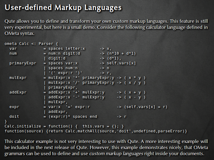
To define a custom markup language, you include an OMeta grammar right inside your document. Such a grammar might look like this.
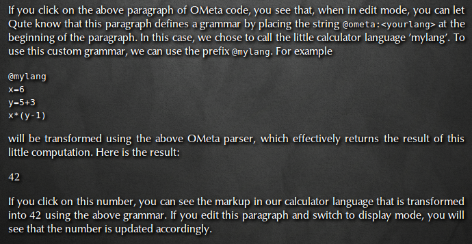
You can then tell Qute that any paragraph in your document is written in the custom language you just defined. Then Qute will transform that paragraph according to the rules specified in the grammar. In this example, we calculate the number 42 by way of OMeta.
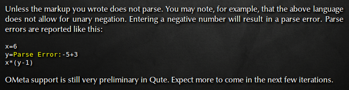
Qute 0.4.1 even supports some rudimentary error reporting.
If you want to try this out for yourself, grab a copy of Qute 0.4.1 from here.
The next milestone is to make this do something interesting. For example, an implementation of Markdown in OMeta would allow the user to easily extend Markdown to suit his or her needs. This is something that I have been missing sorely while writing mathematics with Qute.
It has been out for a while already, but now I finally get around to announcing it here: my first venture into philosophy.
Moshé Feldenkrais’ work and Laozi’s classic, the Daode Jing, have both had a big effect on me and I have always been struck by how alike in spirit these (at first glance) very different philosophies are. In the summer of 2010, I heard a great talk by Steve Palmquist about parallels between the Daode Jing and Kant’s philosophy and this experience gave me the confidence to sit down and work out my own ideas on the relationship between Feldenkrais and Laozi.
The mathematical community is discussing how we can leave the journal publishing model behind us. However, putting journals online, making them open access or even leaving them behind us entirely will not solve the challenges the mathematical sciences face in the next couple of decades. A couple of weeks ago, Peter Krautzberger captured this point of view with the simple and beautiful slogan:
Not beyond Journals, beyond Papers.
I agree! And I would like to go one step further. We have to go beyond journals. We have to go beyond papers. And we have to go beyond that which we, as mathematicians, hold dearest:
We have to go beyond theorems!
In this post, I want to make an argument why, from my point of view. This is going to be a long post, but I will try not to rant too much.
The number of new results per year is increasing
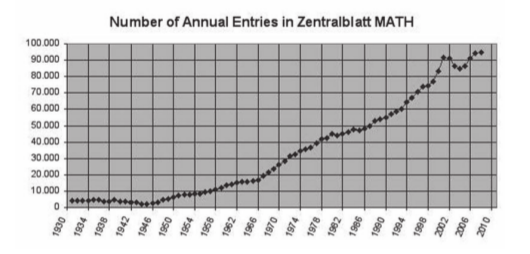
The number of mathematical articles - and theorems! - published each year has increased dramatically in the last decades. To give you just one piece of evidence, here is a graph of the number of new research articles entered in the Zentralblatt MATH index each year. This figure is taken from Bernd Wegner’s article in the June 2011 newsletter of the European Mathematical Society.
This trend will continue. The human population on earth is increasing and (on average) becoming more prosperous. So, more people will pursue an academic career and more people will become research mathematicians. And, because new theorems are the currency in which mathematicians currently measure research activity, this means that the number of new (!) theorems proven each year will continue to increase dramatically - unless we change our way of thinking about research.
This increase is a loss for everyone
There are roughly 100,000 mathematical articles on the Zentralblatt index that have been published in 2010. One hundred thousand articles, of which the majority contain (supposedly) new results. I’d go so far as to say that most mathematicians cannot read and properly digest more than 100 articles per year. (For me personally, the number is certainly lower than that.)
This means that most mathematicians cannot even make use of 0.1% of the new results published each year.
This must have at least one of the following two consequences. In my opinion, it has both.
Mathematical research is becoming more and more specific.
Mathematicians have a great talent for inventing ever more particular fields and sub-fields and sub-sub-fields in which we can discover ever more new theorems. If this strategy is successful, then these theorems are truly new and they have never come up in another area before. The flip side of the coin is of course that the majority of these very particular theorems will simply not be relevant for most mathematicians (and they will be utterly irrelevant for the rest of the world). A favorite objection to this argument is that, a couple of decades down the road, these results will become relevant in other fields and that results from today will be made use of then. But how is this supposed to happen if mathematicians can only read less than 0.1% of what is published this year? It is much more likely that mathematicians who, 20 years later, arrive at an equivalent problem in another field will simply solve it again on their own. Which brings us to the other consequence.
Mathematical research is becoming more and more redundant.
Independent rediscoveries of theorems happen all the time. They may happen more or less simultaneously. Or they may happen a couple of years apart. Or they may happen in entirely different fields, in which case it may take a while for people to notice that these results are, in fact, equivalent. Whatever form these redundancies take, their number is going to increase.
One can make the argument, that this is no problem at all. Science is redundant. So if all a rediscovery achieves is to make an old result popular in a different time or a different area, then so be it! But this clear eyed view of the world goes against the grain of our current self-image as mathematicians, where only original (never-seen-before) theorems count.
Also, redundancy becomes a real problem in conjunction with increasing specialization. What is the point of doing foundational research in a narrow area of specialization today, if the people who may need this stuff twenty years down the road have no means of discovering it? The only insurance against this type of disaster is to focus on advertising our small corner of mathematics, in the hope that somebody will remember it when the time comes. But again, our mathematical community is not built on this socio-dynamic view of research.
In the end, both trends, increasing specialization and increasing redundance, have the same effect:
Mathematical research is becoming increasingly irrelevant.
Note that I am not saying that mathematics is becoming increasingly irrelevant! There will always be seminal theorems that have a far reaching impact on both mathematics and the real world. But the work of the average research mathematician is going to become increasingly irrelevant.
Unless we finally stop to believe that the only valid form of “research” in mathematics is proving new theorems.
Beyond theorems
I have tried to argue above that the business of churning out as many new theorems as possible is not in the best interest of both mathematicians and mathematics. The two causes that I see as central in this regard are the following.
We as a community view only new theorems as research. (Thus we create incentives to produce an unnecessarily large inflation of theorems.)
Our current methods of discovering theorems do not scale with the increase in theorem production.
Thus the best way out of this situation is to acknowledge other forms of mathematical activity as research, not only the proving of new theorems. In particular, activities that help in the discovery of mathematical ideas should be promoted. Here are a couple of suggestions:
Communicating mathematics. This includes all forms of communication, by means of talks, videos, games and of course writing in blog posts, web forums (such as mathoverflow), survey articles and books. This should also include all levels of writing, from expository work for students to references for experts. Finally, this should also include all audiences, from the interested public, to scientists outside mathematics, to mathematicians in other fields and finally specialists in your area. All of these forms of communicating mathematics are widely recognized in the mathematical community. But they are not recognized as research. I argue that mathematicians should get credit as researchers for communicating mathematics, because a larger part of every mathematician’s work will have to be about communication if we are to cope with the present inflation of new results. And we should make it possible that researchers specialize in these social activities, which will only be possible if we give them proper recognition.
Collaborative theorem proving. Instead of everyone trying to get their little theorem published, why do we not try to find new ways of working on the big open questions collaboratively? The polymath projects are very valuable efforts in this regard, but they are only a small first step. As someone on the sidelines of these projects, it appeared to me that in the end, only a relatively small number of people were able to actually contribute to any given polymath project. We have to find ways to make large projects like this asynchronous and distributed. That means, we have to find ways how people can contribute half-baked ideas to research projects, how people who might find them useful can discover them and how to give credit for half-baked ideas in the mathematical community. How to solve these problems is wide open, from my point of view.
The two topics of communicating mathematics and “crowd sourcing” proofs have been widely dicussed in the current debate about mathematical publishing. Now on to two points that have received less attention, as far as I know.
Implementing mathematical software. To make mathematical methods discoverable (and useful), it is of tremendous value to have them implemented in software. This applies to algorithms and methods for visualization as well as to such mundane tasks as the development of decent user interfaces. While these may be engineering tasks in many cases, we should recognize them as research, because they are crucial to the advancement of mathematics! Moreover turning all the useful algorithms available in the literature into usable software is a huge endeavour - it just won’t happen without the proper incentives.
Formalizing mathematics. In my opinion, formalizing mathematics is the single one most important thing that needs to happen if we want mathematics to scale. With “formalizing mathematics” I mean a huge process that includes all of the following.
The development of the languages and tools necessary to make the formalization of mathematical definitions, theorems and proofs feasible for the average mathematician.
This will have to go hand in hand with the development of automatic proof systems that can automatically “fill in the gaps” present in any research article.
The creation of an infrastructure that allows formal mathematical articles to be shared and discovered across different proof systems and formal mathematical languages.
And, finally, the formalization of (almost) all of mathematics.
It goes without saying that this is more than enough work for generations (plural!) of mathematicians. We still have a long way to go in all of the four areas indicated by the four bullet points above. And even though work is going on in all of these areas, this work is not as widely known as it should. Freek Wiedijk was kind enough to give me a brief tour last fall, and I plan to blog about this in the near future.
Here is why I think the project of formalizing mathematics is crucial. We, as humans, cannot cope with the sheer quantity of mathematical output that is going to be produced in the 21st century. So we have to teach computers how to discover theorems for us that are relevant for the questions we are interested in. Otherwise, the work of most mathematicians will disappear into obscurity faster than anyone can be comfortable with.
Communicating mathematics, collaborative theorem proving, implementing mathematical software and formalizing mathematics are of course all closely interrelated. Why should we not dream of composite electronic resources that are accessible and understandable by all kinds of different readers, that we work on collaboratively and that combine expository texts with detailed explanations and usable software with formalized mathematics? This dream is certainly not new and it is shared by many. How should this brave new world of mathematics look like in detail and how do we build it? The process of exploring these questions will be interesting indeed. My point here is that to get there we need to give up the belief that theorem proving is what mathematical research is all about.
The self-image of the mathematician
No matter what happens, proving mathematical theorems is going to become less relevant. If we succeed in changing they way mathematical research works, other activities will become more important. If we do not, the theorems most mathematicians prove will, generally, be redundant and overspecialized. So:
Theorems will become less relevant.
The social and psychological impact of this simple observation is huge. The self-image of the modern mathematician is built entirely on proofs and theorems. We, as mathematicians, grow up on stories of great “heros” who became “immortal” by proving all these great theorems we learn about. Naturally, we aspire to do as they did and so we seek to wrest these eternal truths from the world of pure, abstract ideas that we conquer using nothing but our “beautiful mind”.
Of course I am being ridiculous here, I exaggerate. But our identity as mathematicians is based on the stories we tell each other about other mathematicians - and those stories revolve around theorems and proofs. Often the only thing we know about a mathematician is what theorem they proved and we set up Millenium Prizes to celebrate the act of attaching a particular mathematician’s name to a particular theorem.
The association of “being a mathematician” with “proving a new theorem” is so tight that I have serious doubts about whether we as a community will accept other mathematical activities as research anytime soon. To do so would call into question what a mathematician is at a fundamental level. But this is precisely what we have to do.
Conclusion
The current model of doing mathematics is in need of reform. The fundamental issues with the current model cannot be resolved just by placing mathematical journals on a different economic and organizational basis. The core of the problem is our fixation as a community on theorems and proofs. As these notions are tied so closely to our self-image as mathematicians, finding a new model of doing mathematics is going to be a long and arduous process. But we have to do it, if we want our work to be relevant in a couple of decades.
One week ago, my most recent math paper appeared on the arXiv and now I finally get around to blogging about it.
The \(f^*\)- and \(h^*\)-coefficents of a polynomial \(p(k)\) are simply the coefficients of \(p(k)\) with respect to certain binomial bases of the space of polynomials. If \(p\) is of degree \(d\), then they are given by \[p(k)=\sum_{i=0}^d f^*_i {k-1 \choose i} =\sum_{i=0}^d h^*_i {k+d-i \choose d}.\]
Where do these definitions come from? The motivation is Ehrhart theory. Given a set \(X\subset\mathbb{R}^d\), the Ehrhart function \(L_X\) of \(X\) is given by \[L_X(k)=\#\mathbb{Z}^d\cap k\cdot X,\] for \(1\leq k \in \mathbb{Z}\), that is, \(L_X(k)\) counts the number of integer points in the \(k\)-th dilate of \(X\).
Now, a famous theorem by Ehrhart states that if \(X\) is a polytope with integral vertices, then \(L_X\) is a polynomial. More precisely, there exists a polynomial that coincides with \(L_X\) at all positive integers and by abuse of notation, we will denote this polynomial by \(L_X\) as well.
After this preamble you may already have guessed it. The binomials in the expansion above are Ehrhart polynomials of particularly nice polytopes, namely half-open unimodular simplices. We denote by \(\Delta^d_i\) the \(d\)-dimensional standard simplex with \(i\)-open faces, i.e., \[\Delta^d_i = \{ x\in\mathbb{R}^{d+1} \;|\; x_0,\ldots,x_{i-1} > 0, x_i,\ldots x_d\geq 0 \sum_{i=0}^d x_i = 1 \} \]
and then it is not hard to check that \[L_{\Delta^d_i}(k) = {k+d-i \choose d}\] and in particular \[L_{\Delta^d_{d+1}}(k) = {k-1\choose d}.\] Thus:
If \(P\) is a lattice polytope with a shellable unimodular triangulation \(K\), then \(h^*_i\) counts the number of \(d\)-dimensional simplices with \(i\) open faces in a shelling of \(K\).
If \(P\) is a lattice polytope with a unimodular triangulation \(K\), then \(f^*_i\) counts the number of \(i\)-dimensional faces in \(K\).
In particular, if \(P\) is sufficiently nice, then both the \(f^*\)- and the \(h^*\)-coefficients are non-negative. The point of my article is to show that even if \(P\) is not nice and partitioning \(P\) into unimodular simplices does not work at all, the \(f^*\)-vector is still non-negative.
Theorem. If \(P\) is a polytopal complex, then the \(f^*\)-coefficients of \(L_P\) are non-negative integers, even if \(P\) does not have a unimodular triangulation.
This becomes relevant when \(P\) is not-convex. As long as \(P\) is a polytope, its \(h^*\)-coefficients are non-negative by a famous theorem of Stanley. However, the \(h^*\)-coefficients of polytopal complexes may well be negative. For example, in recent work, Martina Kubitzke, Aaron Dall and myself have shown that there exist coloring complexes of hypergraphs with negative \(h^*\)-coefficents.
In fact, we can take this theorem one step further and use it to characterize Ehrhart polynomials of what I call partial polytopal complexes. An integral partial polytopal complex is any set in \(\mathbb{R}^d\) that can be written as the disjoint union of relatively open polytopes with integral vertices.
Theorem. A vector is the vector of \(f^*\)-coefficients of some integral partial polytopal complex if and only if it is integral and non-negative.
Behind all of this lies a combinatorial interpretation of the \(f^*\)-coefficients in a (not necessarily unimodular) lattice simplex and a new way of partitioning the set of lattice points in a simplicial cone into discrete cones.
For more results, in particular about the rational case, and more details on all of this, please check out my article! It has the id arxiv: 1202.2652.
This fall semester, I taught the Math 890 course at San Francisco State University. It was the very first course that I taught all on my own. I am currently funded by the DFG, so I have no teaching obligation (in fact, I had to ask the DFG for permission to devote my time to something other than research). But when I was offered this opportunity, I leapt at the chance and volunteered to teach this course, even though, with two 75 minute classes each week, it was a significant amount of work. I wanted the experience, and, after all the years where I was responsible only for my own research portfolio, I was looking forward to taking on some real responsibility. Also, this was a topic course for graduate students, so that I could teach anything that I wanted. What a wonderful opportunity to experiment!
In this post, I will present the idea behind the course I gave, give an outline of the topics covered, provide all my slides and notes for the lecture as well as all the exercise problems, give a list of topics for the seminar, and review how the course, as a whole, went.
Note: The material linked below is known to contain a number of typos.
The Idea
I always wanted to try a different format of a course. With “format” I do not mean the methodology for teaching - experiments in that department are certainly called for, but I wanted to stick to the classical lecture + seminar format (because I actually enjoyed it as a student). What I wanted to experiment with was the content of my course.
Math courses, the way I experienced them at the FU Berlin, typically build a theory from the ground up, in a very detailed fashion. They emphasize rigor over intuition, and have a classical definition-theorem-proof structure. Courses of this “classic” format are certainly important, especially for teaching mathematical rigor, but here, I wanted to do things differently:
The course was to cover a large range of topics, with the aim of showing their interconnections,
intuition was to be emphasized over rigor,
and it was to make extensive use of visualization.
In short, I wanted to give my students a grand tour of the mathematics that I find interesting. Adding courses of this type to the curriculum is important for a number of reasons. I do not want to go into too much detail on this, so here are just a few bulletpoints, in no particular order.
For me personally, grand tours are simply more inspiring than develop-a-theory-from-the ground-up-lectures. I want to take a grand tour of the house, instead of spending my time laying bricks for the foundations!
Grand tours have more room to present applications of the covered material.
Pure mathematics especially are not measured only in terms the applications they have. The beauty, insight and perspective they have to offer are of direct value to us as human beings. However beauty, insight and perspective are tied primarily to the rough ideas and much less to the technical details. So let’s cover more beautiful ideas and less details!
Showing the connections between different fields make all of these fields more relevant to the audience!
First, I cannot remember a theorem unless I develop some kind of intuition for it. Second, I cannot prove similar theorems on my own, without having an intuitive idea why it should be true. Third, the intuitive idea is often all I remember off the top of my head after a couple of weeks have passed. So why not focus on teaching the intuition in the first place?
For me personally visualization is by far the best way to develop an intuition.
Outline
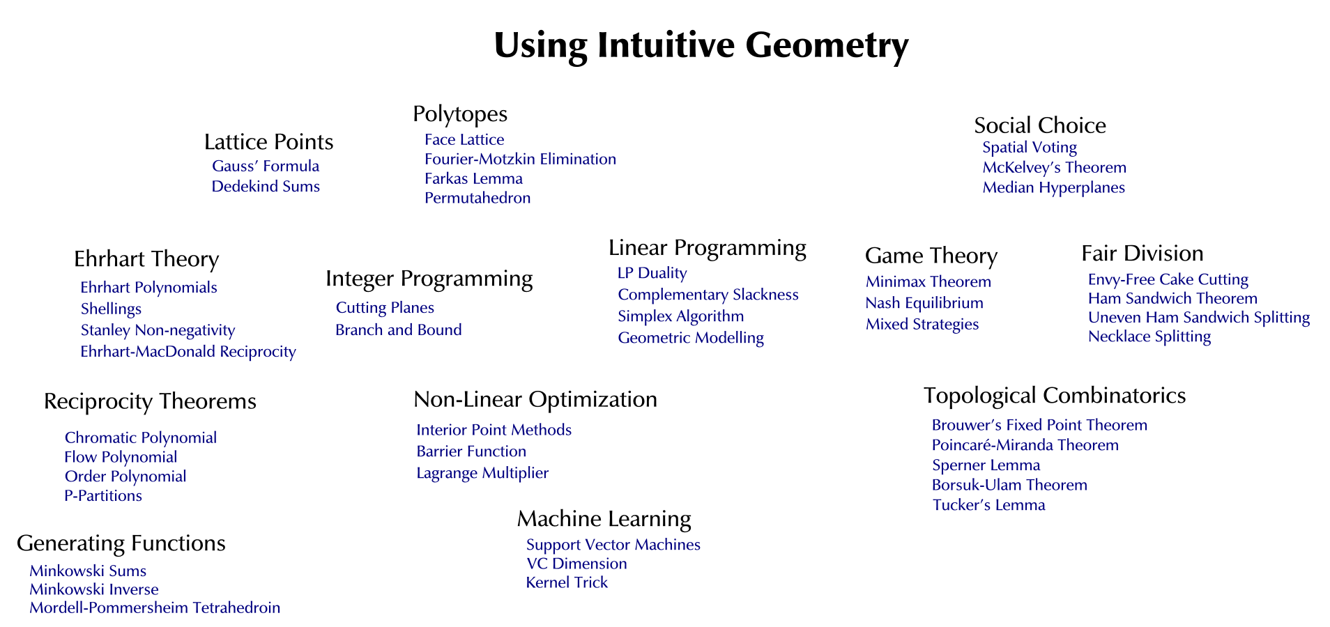
The topics that were covered in the lecture + seminar are show in the big mind map at the top of this page. As you can see, the variety of topics is very large. Each of the big headlines in the mindmap could easily make up an entire course on its own! All of these topics are interrelated. Yet, it is hard to come up with a single title for the course that includes them all. “Discrete Geometry”, certainly, is too generic and not entirely accurate. In the end, I decided to call the course:
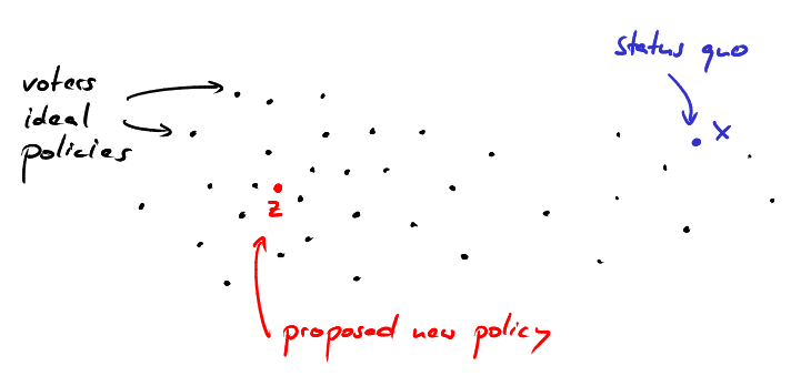
Using Intuitive Geometry - Using Geometry Intuitively
I like this title, because it makes clear that I care more about methods and intuition, than about giving a comprehensive account of anything. For example, Game Theory is certainly no subset of Discrete Geometry, but methods from “intuitive geometry” do play a big role: The Minimax Theorem in Game Theory is both equivalent to the LP Duality Theorem and it is implied by Brouwer’s Fixed Point Theorem, which are both staples of intuitive geometry.
In hindsight, it occured to me that another fitting title would have been:
Adventures with Hyperplanes
Well, maybe next time. Here are the slides and notes from the tour I took this fall through all of these diverse topics:
Visualizing Numbers
(Gauss sum formula, lattice points in triangles, staircases, Dedekind sums)
After 10 weeks of lectures, we had 4 weeks of student talks. Some of the talks were in-depth talks on a particular subject, while others were brief introductions to large subject areas. These are the topics I suggested:
The Mordell-Pommersheim Tetrahedron. (Source: Computing the Continuous Discretely. Beck, Robins. 2007. Chapter 8.)
Power Indices and Spatial Power Indices (Source: Power and Stability in Politics. Straffin. In: Handbook of Game Theory Volume 2. Chapter 32. 1994.)
Interior Point Methods (Source: The integer-point revolution in optimization: History, recent developments, and lasting consequences. Wright. 2004. link)
The Borsuk-Ulam Theorem and Ham Sandwich Splitting (Source: Using the Borsuk-Ulam Theorem. Matousek. 2003. Chapters 2 and 3.)
Integer Programming Methods (Source: Theory of Linear and Integer Programming. Schrijver. 1986. Chapters 23 and 24.)
I am very happy with how the course turned out! This “grand tour” style of a course succeeded in engaging the students. From what I heard, my students not only learned something, but also took away a new perspective on many of the subjects I covered. One student even told me that they now had a much better understanding what the thesis they had been working on is about. Was will man mehr!
Nonetheless there are of course a number of things I would like to improve the next time I teach this course - which I would really like to do! Here is a list of notes that I would like to keep in mind for the next iteration.
Exercises
The exercises were what made this “intuitive tour” type of course work. Had my students not spent the time to accquaint themselves personally with the subject matter, I guess many parts of this course might have remained too vague. The great thing is, that my students did work through virtually all of the exercise problems, even though I did not have the resources to grade the correctness of their solutions. It would have been too easy to skip corners - but they didn’t! Thus, I really have to thank them for their initiative, curiosity and dilligence - they made this course work (even more than ususal)!
In hindsight, I think this large program is better suited to a course with three 75 minute sessions per week. Two sessions for lectures and one for talking about the exercise problems. Also, it would have been very valuable to provide individual corrections for the exercises and/or solutions of the exercises for the students to review on their own.
Lecture Notes
I wrote the script for my lectures as I went along. Given that the material was so diverse and scattered over so many sources and given that it was my ambition to present some material from an (AFAIK) original perspective, this was very work intensive. Originally, I had planned to use my blog to record detailed lecture notes, but this turned out to be infeasible. (Currently, it takes me at least four hours to write up notes for one 75-minute lecture in a form suitably self-contained for a blog post - even if I have prepared the material beforehand in slide form and given the lecture in front of class. Is that typical or somewhat slow?)
The points mentioned so far (publish lecture notes, publish solutions for the exercises, provide individual corrections for the exercises) all boil down to putting in more work. And when I give this course the next time, I certainly want to prepare lecture notes and solutions beforehand and work together with a teaching assistant for grading! Here are some more thoughts, though, that take a different direction:
Seminar
Combining the lecture with a seminar was an excellent choice. For two reasons. First, it gave the students the opportunity to work on a subject in depth. This was especially important as the “intuitive tour” format (by necessity) left the students wanting more details. The seminar gives students the opportunity to pick one subject they find particularly appealing and dig into the details that were only hinted at in the lecture and in the exercises.
Second, the seminar was enjoyable not only for the students, but for me as well! During preparation, it was simply fun to get together and puzzle about a problem or figure out the best picture for illustrating a theorem. (Especially after I had spent hours on end with mainly one-way communication during the lecture.) On the whole, the talks were very good and got across all the important points. Some even went above and beyond the suggested material! Next time, I might be tempted to make the seminar a much bigger part of the course!
Proofs
What place do proofs have in this type of course? After the first two weeks of the course I become worried that my intuitive style of lecturing might be too vague for my audience. This worry was not fed by any actual observations during class, but rather by my rookie-lecturer-confidence wavering. So I decided to up the level of detail in the next few weeks and include more proofs and a greater level of formality. In retrospect, after talking with my students about it and judging from the their exercise solutions, I can say that this failed completely. This “proofy” part of the lecture was the part my students enjoyed the least and it was the part they had the least grasp of, judging by the exercises. (Of course, proper lecture notes would have helped their performance in the exercises, but I think this is not the main point here.)
I was reminded here of these great quotes by Victor Klee:
“A good talk contains no proofs; a great talk contains no theorems.”
“Mathematical proofs should only be communicated in private and to consenting adults.”
In any case, they have no place in this type of lecture! Intuitions for why a theorem should hold, rough proof sketches, all of these certainly belong in this type of lecture. But going the extra distance from an intutive proof sketch to an actual “formal” proof is not worth it - simply because any formalization is significantly harder to understand than the intuitive idea that gave rise to it. If your goal is to teach a theory, then teaching that formalization is part of what you want to communicate. If your goal is to show connections between different fields intuitively, then that formalization is only tangential to what you want to communicate. So, adding formalism just for the sake of communicating an intuitive idea is not going help - instead of clarifying the point it will obfuscate.
Of course this does not mean that proofs are irrelevant! On the contrary, if students are to learn how to use geometric intuition, then learning how to make intuitive ideas precise is crucial. However this is an active process. Students have to do it themselves when solving exercises or preparing seminar talks. My doing it at the whiteboard does not help anybody! More precisely: my doing it at the whiteboard helps only, if students have tried to do it by themselves beforehand.
I will not try to write down here all the mental notes I made for myself on how to present proof ideas if you do not want to make them 100% precise. (Maybe I will write another blog post about this.) I want to mention two things, however: First, when explaining an algorithm/constructive proof it is much more important to make the construction precise and illustrate it with an example than to prove its correctness. Second, always give a concise summary of the key point of a theorem or proof that you just explained. That way, even those members of your audience that you may have lost will have something concrete to remember.
Drawing
Of course, when talking about geometric intuition, drawing is the most important thing! Two shorts thoughts about this:
The most important aspect of many mathematical figures is the way they are drawn and not the final image. Thus it is very important to construct a figure slowly, step by step. No fancy visualization tool beats a good drawing on a whiteboard!
In this vein, I encouraged my students to draw the objects they were talking about, both in the exercises and in the seminar - and I got everybody to do it in the end! I was very happy about this, because, in my opinion, drawing is an essential skill for any mathematician!
Conclusion
It was a great experience teaching this course! I learned a lot, both in terms of hard skills and soft skills. I would love to teach this course a second time, and the next time I would like to experiment more with teaching methodology. Also, I would really like to write up this tour through some uses of intuitive geometry in book form and smooth out all the wrinkles along the way. But, maybe, the printed page (or static PDF document) is just not the right medium for this.
I think mathematics could benefit from more courses and texts of this “intuitive tour” type: overview material with a strong emphasis on intuition and visuals, accessible to advanced undergraduates but with enough depth to satisfy graduate students.
Bibliography
Finally, here is a short informal summary of the literature I used for the preparation of this course.
Beck, Combinatorial Reciprocity Theorems.
Beck, Robins, Computing the Continuous Discretely.
Bisschop, AIMMS Optimization Modelling.
Breuer, Heymann, Staircases in , Integers.
de Longueville, A Course in Topological Combinatorics.
Gaiha, Gupta, Adjacent Vertices on a Permutohedron, SIAM Journal on Applied Mathematics.
Grötschel, Lineare und Ganzzahlige Programmierung.
Matousek, Using the Borsuk-Ulam Theorem.
McKelvey, Intransitivities in multidimensional voting models and some implications for agenda control, Journal of Economic Theory.
McKelvey, General Conditions for Global Intransitivities in Formal Voting Models, Econometrica.
Raghavan, Zero-sum two-person games, Handbook of Game Theory, Vol 2.
Schölkopf, Smola, Learning with Kernels.
Schrijver, Theory of Linear and Integer Programming.
Straffin, Power and stability in politics, Handbook of Game Theory, Vol 2.
Wright, The interior-point revolution in optimization: History, recent developments, and lasting consequences, Bulletin of the American Mathematical Society.
These are notes for a talk I gave both in my course at SF State and at the teach-in against police violence at UC Berkeley. The talk at the teach-in found its way on IndyMedia and YouTube (Pt 12).
In a democracy, people are fighting all the time over control of the political agenda. Media campaigns, protests and lobbying are all examples of people trying to shape the political discourse. They seek to get “the public” to discuss a topic they care about, they seek to shift the focus of the current political discussion towards the points they think are important or they may even want to throw up a smokescreen to divert the public from a topic they consider dangerous for them. This process is vital for a democracy to work. In fact, I want to present a mathematical argument that supports the following bold claim: This process is more important for a democracy than voting! And perhaps the most amazing thing about this observation is that this is a direct consequence of the geometry of voting.
Policies as points in space
Political choices can often be represented by points in space. By this I mean that often, all the different policies that can be adopted with regard to a given political issue can be represented by different points in space.
As an example, let us consider budget decisions. A state’s budget can be represented by three numbers:
the state’s revenue (e.g. taxes)
the state’s expenditures (e.g. public spending)
the state’s deficit
In this way, we can view every possible budget decision as a point in three-dimensional space. However, these three values are not independent of each other. Instead they are related by
deficit = spending - taxes.
This equation defines a plane in three dimensional space. All possible budgets lie in this hyperplane. To visualize how this looks consider the following three dimensional coordinate system. The axes represent spending, taxes and deficit. The budget hyperplane lies slanted in space. Its intersections with the three coordinate hyperplanes are shown as dashed lines. For example, the horizontal dashed line is the set of budgets with spending = 0. It is a diagonal in the plane spanned by the deficit and taxes axes. Similarly, the other two dashed lines are diagonals in the deficit/spending and spending/taxes coordinate hyperplanes.
As we have seen, the set of all budgets with spending = 0 forms a line in the plane of all possible budgets. Increasing or decreasing spending by, say, 1 dollar corresponds to translating this line in the plane. Taking all translates by $k$ dollars, we obatin a family of parallel lines. And if we repeat this for the lines given by taxes = 0 and deficit = 0, we obtain a triangulation of the budget plane as shown below.
This picture shows a part of this triangular lattice. It allows us to visualize what happens if we change a given budget $b$. Say $b$ is given by a spending of 3 trillion dollars, tax revenues of 2 trillion dollars and a deficit of 1 trillion dollars and suppose we increase tax revenues by 1 dollar. This corresponds to moving from $b$ to the line given by 1 trillion and one dollar of tax revenues. However, we have to make a choice here. Do we use that one extra dollar to lower the deficit or increase spending? If we go “left” in the picture, we stay on a line where the deficit remains constant but we move from one “spending line” to the next thus increasing spending. On the other hand, if we go “right” we keep spending constant and decrease the deficit.
Now that we have a means to visualize how different budget decisions relate to each other, we can use that to visualize the current positions of various political actors in the US with regard to the federal budget.
We place the 2011 federal budget in the center of our picture at the point labeled $b$. Next we draw the three lines through $b$ along which spending, taxes and deficit are constant, respectively. Both, the democrats and the republicans want to decrease the deficit. So if you asked a democrat or republican where their ideal 2012 budget would be, then they would tell you that it lies below the deficit line through $b$. Ideally, however, a democrat would like to decrease the deficit by increasing taxes, without decreasing spending. So, qualitatively, a democrat’s ideal policy would lie in the blue region. A republican, on the other hand, would want to reduce spending to finance the decrease in deficit without raising taxes. So a republican’s ideal policy would lie in the red region. There are other people, though, e.g., Keynesian economists, who think that lowering the deficit is not a priority at the moment. They think that it is much more important to stimulate the economy by lowering taxes and increasing spending, even if that means that the deficit has to increase even further. People in this comparatively small group might have an ideal budget somewhere in the green region.
We have now seen how to think geometrically about politics. Now we are going to apply this point of view to analyze the dynamics of the majority vote.
Spatial Voting and the Power of Agenda Control
So far, we have only visualized policies as points in space. Now we come to McKelvey’s theorem, the main result I want to tell you about. To be able to state this theorem, we need to formulate a model of voting, called spatial voting.
As we discussed, every policy corresponds to a point in space. Now, spatial voting simply means the following.
Voters are asked to decide between two alternatives, the status quo which we call $x$ and a proposed new policy $z$. Voters can vote for either of these two alternatives.
The alternative with the most votes wins, i.e., we are having a majority vote.
Every voter has an ideal policy in mind. So the voters can be represented by a set of points in space.
Finally, we make a very important assumption: Every voter will vote for the alternative closest to his or her ideal policy!
Consider as an example the following picture. The black points represent the ideal policies of all voters. The blue point labeled $x$ marks the status quo, while the red point labeled $z$ marks the proposed new policy. In this example, most voters are going to vote for $z$ as $z$ is closer to their ideal than $x$. As we are running a majority vote, this means that $z$ is going to be approved and will become the new policy.
Now we can state McKelvey’s theorem.
Theorem. (McKelvey 1976) For every status quo $x$ and every other policy $z$ there exist policies $y_1,y_2,\ldots,y_k$ such that
$x$ loses against $y_1$ which loses against $y_2$ which loses against $y_3$ … which loses against $y_{k-1}$ which loses against $y_k$ which loses against $z$
in the majority vote.
What does this mean? Suppose there were someone with complete control of the agenda. This agenda controller would have absolute control over which new policies are proposed. Whenever the agenda controllers proposes a new policy, the voters would get to vote and the agenda controller would be bound by their decision according to the majority rule. This means that an agenda controller cannot decide anything. All he can control is between which alternatives the voters get to choose.
So, suppose there is an aganda controller and the current status quo is $x$. Suppose further that the agenda controller wants voters to pass a new policy $z$ that he favors (but that everybody else may hate). McKelvey’s theorem now states that there are cleverly devised policies $y_1,\ldots,y_k$ such that the agenda controller can proceed as follows. First, he proposes $y_1$. The voters get to choose between $x$ and $y_1$ and they approve $y_1$ as the new policy because the majority of voters prefers $y_1$ to $x$. Now $y_1$ is the new status quo. Next, the agenda controller proposes $y_2$ and again, the voters prefer $y_2$ over $y_1$ so they are going to adopt $y_2$ as the new status quo of their own free will. The agenda controller continues in this fashion until the voters pass $y_k$ as their new policy. Then he makes his final move and proposes $z$, the policy that he likes but that everybody else hates. However, through his previous moves, he has managed to put the public in a position where the majority actually prefers $z$ to the current status quo $y_k$. And so they are going to approve of $z$ of their own free will.
In this way, someone in control of the political agenda is in complete power, even if he is bound by the majority vote of the population. This explains why, for example, freedom of speech and the right to protest are so important parts of democracy. Protest is a way of getting a certain item on the political agenda, trying to influence the direction that current policy should take. (See here for a recent example.) Conversely, if there is a small elite who dictates the political topic of the day, then this elite will get its way, no matter if vote or not. So the morale of the story is this:
Voting alone does not give the people any power! Just by voting, you can’t control anything. You also have to have a public discussion about political topics and this is what protest is about.
At this point, it is important to stress the difference between the provocative morale that I drew from the story and the statement of the original theorem. The theorem is provably true, but applies only to a very specific abstract model of a society. In reality, no one is in absolute control of the political agenda! And the theorem tells us that this is a very good thing!
So, while the theorem does not apply to western democracies such as the USA, it can still tell us something about the real world, by way of analogy, in just the same way that a good novel can reveal a truth about the world we live in. (See the Q&A section for more about this.)
Now that we have both a formal as well as an intuitive feeling of what McKelvey’s theorem is saying, let us try to get an idea why the theorem should be true.
The Idea behind McKelvey’s Theorem
In this section, I want to give an idea how the sequence of policies $y_1,\ldots,y_k$ are constructed. If you want, this is a proof by example, but of course it is not a complete proof of the theorem. For a thorough proof I refer the interested reader to the literature cited at the end of the Q&A section.
We work with an example in 2 dimensions. There are three voters $v_1,v_2,v_3$ whose ideal policies are given by the three black points $p_1,p_2,p_3$ in the picture. We draw the lines through any pair of these three points. The status quo is given by the blue mark in the center of this triangle formed by the voters’ ideals. So, intuitively, the current status quo $x$ seems like a pretty good compromise between the voters’ preferences.
Which policies defeat the status quo $x$ in a majority vote? Remember that the three voters will vote for the alternative closest to their ideal policy. So, for each voter, we draw a circle around that voter’s ideal policy and we choose the radius of that circle such that the cirlcle passes through the status quo $x$. Let $C_1$ be the circle around voter $v_1$’s ideal policy $p_1$. $v_1$ will prefer any policy $y$ to $x$ that lies strictly inside the circle $C_1$!
Consequently, the policies that will defeat $x$ lie in the intersection of any two of the circles shown in the picture. The area corresponding to the set of policies that defeat $x$ are shaded green in the picture. As you notice, the shaded area extends outside of the triangle spanned by the three ideal policies $p_1,p_2,p_3$. Let $L_1$ denote the line through $p_1$ and $p_2$. If we reflect $x$ at $L_1$, then we will obtain a point $x’$ at exactly the same distance to $p_1$ and $p_2$ as $x$. If we now move $x’$ inwards for a little bit, the resulting point $x”$ will lie strictly in the interior of both $C_1$ and $C_2$. Thus $x”$ will defeat $x$ in a majority vote, because both voters $v_1$ and $v_2$ will like $x”$ slightly bettern than $x$. Note, however, that for $v_3$ the new policy $x”$ is much worse than the status quo $x$. Since we are working with a majority vote, however, this is not taken into account.
As it turns out, this construction always works! We summarize this observation as follows.
For any policy $x$ and any line $L$ through two of the voters’ ideal policies, the policy $x”$ obtained by first reflecting $x$ at $L$ and then moving the reflected point back towards $L$ a tiny bit, will always defeat $x$ in a majority vote. Typically, $x”$ will be “slightly better” than $x$ for two of the voters and much worse for the third voter.
This observation is the staples of the agenda controller’s strategy for manipulating the voters. Phrased provocatively, the agenda controller’s strategy is this:
Play off different groups of voters against each other! Offer a majority of voters marginal incentives to hurt a minority really bad!
So how can an agenda controller use this strategy to get voters to vote for his favorite policy? The following figure tells it all.
We start with a status quo $x$. This we reflect $x$ along the line $L_1$ through $p_1$ and $p_2$ by playing off voters $v_1$ and $v_2$ against voter $v_3$ to get to a new policy $y_1$. Next, we reflect $y_1$ along $L_3$ by playing off $p_1$ and $p_3$ against $p_2$ to get to $y_2$. Then, we reflect $y_2$ along $L_2$, by playing off $p_2$ and $p_3$ against $p_1$. We can keep going in this fashion as long as we like. Note that in each step we give two of our voters a tiny improvement (we move towards their ideal points by a tiny bit) while at the same time making the situation much worse for the third one (we move much further away from his ideal policy). In total, we make the situation worse in every step! So if we continue this process long enough, everybody will be so unhappy with the current policy ($y_k$ will be so far away from all voters’ ideal policies) that everybody will be happy to agree to the policy $z$ that the agenda controller had in mind all along.
I find this proof striking for a number of reasons. First of all, even from this small example, you get a clear idea how the proof will proceed in the general case (even though you need a couple of technical tools like median hyperplanes). Second, for three voters, the proof requires only an elementary geometric construction that (I hope) does not scare off people who do not feel that comfortable around mathematics. Finally, and this is most remarkable, this proof gives clear instructions how someone who wants to manipulate public decision making should go about it: Play off different groups of voters against each other! The fact that many political decisions are two or higher dimensional provides the necessary room to maneuver.
(In fact, I find it striking how similar the manipulative stragtegy suggested by the geometry of voting is to how many agents on the political stage actually behave. To manipulate public opinion, they try to reduce the public discussion on an issue to a one-dimensional problem. To a choice between two alternatives. They try to hide the fact that real world problems are higher-dimensional.)
Conclusion
I hope to have convinced you that there is merit in looking at politics from a geometric point of view. A natural consequence of this point of view is McKelvey’s theorem, which states that an agenda controller can get voters to agree to anything the agenda controller wants of their own free will. Fortunately, there are no perfect agenda controllers in real world democracies! But McKelvey’s theorem reminds us that we had better exercise the freedom we have to shape the political agenda. Because without active political debate, the right to vote alone does not give the public any power at all.
Q&A
There are a great many things more to say about all this. Here are a few of them.
Budgets are more complicated than this!
Of course a state’s budget is much more complex than the model I suggested above. There are many more parameters to take into account! The advantage of this model is that it captures the gist of the problem while still being low-dimensional enough so that we can draw something!
There are some assumptions missing from McKelvey’s theorem!
That is true. First of all, McKelvey’s theorem only works in dimensions two and up. If different policies all lie on a line, then McKelvey’s theorem fails. The same thing can happen in higher dimensions if the voters’ individual preferences have a particular pattern. For example, if all voters have the exact same ideal, then agenda control won’t work. The technical assumption I omitted in the above statement, is that the median hyperplanes (whatever that is) of the the voters’ ideal policies do not all intersect in a single point. However, this assumption is not critical for the following reason: By slightly perturbing the voters ideal policies we can always guarantee that this assumption is satisfied. Also, the theorem assumes that the set of policies is all of $\mathbb{R}^n$. This is not true in the budget example, as negative values for taxes or spending do not make sense (a negative deficit is fine, though). But generalizations of McKelvey’s theorem take care of this issue (see below). Finally, the theorem assumes an odd number of voters. McKelvey argues, however, that this makes no difference, as the agenda controller can decide to participate in the vote if and only if his vote is required to make the total number of votes odd.
It should also be mentioned that McKelvey’s theorem assumes that all voters use the Euclidean distance to measure which policies they prefer. However, this assumption is not essential as McKelvey showed in a subsequent paper. (See below.)
What generalizations of McKelvey’s theorem are there?
McKelvey generalized his theorem considerably in subsequent work. For example, he showed that if the set of policies is an arbitrary connected subset $X$ of $\mathbb{R}^n$ and each voter measures with his or her own, private notion of distance (which has to be continuous) then, still, the top cycle of the majority rule is going to be all of $X$ (i.e., agenda control works). He concludes, in his own words:
“Regardless of other voters’ preferences, any one voter with complete information of the other voters’ preferences, control of the agenda, and the ability to cast his own vote as he chooses can always construct majority paths to get anywhere in space.”
Is protest really more important than voting?
The provocative catchphrase that “protest is more important than voting” is meant in the following sense: A political system in which people do not shape the political agenda at all but only go to vote is not democratic. In this sense, active participation in the public political discourse is at least as important as going to vote. This is not to be construed as an excuse not to go voting, however!
Is there a mathematical proof that influencing the political agenda is more important than voting?
No. Mathematics makes statements about abstract models. McKelvey’s theorem makes a statement about a particular abstract model of a society in which the people do not influence the political agenda at all and behave in a predictable way. This statement is provably true. But “mathematics” makes no claim whatsoever about what this statement about an abstract model has to do with reality.
How realistic is the model of society assumed in McKelvey’s theorem?
First of all: I am not a political scientist, and I do not know of any empirical research on this subject. My personal opinion, however, is the following: Western democracies such as the USA do not fit the model of McKelvey’s theorem at all. In particular there are a number of important differences:
In practice, all actors on the political stage constantly strive to control the agenda! So McKelvey’s theorem does not apply to practical politics, but it offers an unconventional explanation why control of the agenda is so strongly contested.
The theorem assumes that the agenda controller has complete information about the preferences off all voters. This is not true in practice. However, never before was so much data about personal opinions readily available to anyone with an internet connection. So one could argue that western societies are converging on the condition required for McKelvey’s theorem to apply.
Voters oppinions change over time. The theorem assumes that opinions are constant. I would guess, though, that the theorem could be extended to account for changing opinions.
There are few voting processes where voters only decide to aprove or reject a single proposition. Presidential election in the US fit this description but are too closely tied to personality to admit a reasonable parameterization by points in space. In most other public elections, the voters have to decide between many alternatives, so spatial voting does not fit either. In process of passing a bill in congress fits the model accurately, however there voters are constantly trying to control the agenda. Ballot propositions also fit the model, but again, voters have direct influence on the available propositions through the initiative system.
As mentioned above, the theorem makes a couple of additional technical assumptions. However, I do not think that these are essential, especially with regard to McKelvey generalizations of his theorem.
There is one technical assumption that deserves special mention: continuity. I do not think that it is that much of a constraint to assume that voters preferences are continuous. Rather, I think it is a significant departure from reality to assume that the space of all policies is a continuum in the first place. For a budget, this is simply false: Two budgets cannot differ infinitessimally - they can only differ by cents.
So, while McKelvey’s theorem does not prove anything about real world democracies, I think it still provides insight on how democracies work.
There is no policy that cannot be defeated by any other policy in a majority vote, right?
Exactly! But instead of looking for a policy that cannot be defeated, we can go for the policy that is least likely to be defeated! This is the policy for which the shaded green area in circle picture above is smallest. As it turns out this so-called “strong point” of the majority game lies roughly in the center of all voters’ ideal points. More precisely, it is given by a convex combination of the voters’ preferences, where the weights of the convex combination are given by spatial power indices of the voters. This means that centrist voters have more influence on the strong point than extremist voters. (Owen and Shapley 1989)
Where can I read more on this?
I recommend the excellent article by P.D. Straffin Jr. in the Handbook of Game Theory and Richard McKelvey’s original articles on the subject.
Straffin, P. D. J. (1994). Power and stability in politics. Handbook of Game Theory with Economic Applications Volume 2 (Vol. 2, pp. 1127-1151). Elsevier.
McKelvey, R. D. (1979). General Conditions for Global Intransitivities in Formal Voting Models. Econometrica, 47(5), 1085-1112.
McKelvey, R. D. (1976). Intransitivities in multidimensional voting models and some implications for agenda control. Journal of Economic Theory, 12, 472-482.
I was shocked by the violence the police here in the Bay Area used against peaceful protesters in recent weeks. Examples include shooting grenades at people lying on the ground and using batons to savagely beat up people for no reason. Apart from being incredibly brutal, I think this kind of police behavior is completely unnecessary and simply unprofessional. It is a vital feature of a democracy that people can protest! And even if camps of protesters need to be removed, there is no reason to use violence to do it!
Last week, Nathan Ilten had the great idea of organizing a teach-in against police violence. Basically, this is a bunch of mathematicians giving lectures in public where everybody can see them. I think this is a great way of raising public awareness for a political issue while at the same time communicating interesting ideas. I have participated in a couple of these in Berlin - we had a lecture in front of the Rotes Rathaus and a lecture in the U-Bahn - and it is great that Nathan took the initiative to make this kind of event happen in Berkeley as well.
The teach-in took place yesterday from 11 to 5 at Dwinelle Plaza on the UC Berkeley campus and it was a resounding success. At the peak, the talks drew crowds of about one hundred people and we had a solid attendance throughout the day. Everything stayed peaceful and we had no trouble with the police at all. (I guess they were busy trying to stare down the people at the Occupy camp on Sproul.) And our event was covered by a local radio station.
We had a wide range of talks, some addressing mathematical aspects of politics, some focusing on mathematical subjects, some targeted at a general audience and some intended for math majors. Our speakers were Chris Manon, Andrew Critch, Charley Crissman, Eugenia Rosu, Piotr Achinger and myself. I do not intend this blog post to be a comprehensive account of the teach-in, so please forgive me when I do not summarize each of their talks. I just want to mention that I particularly enjoyed Andrew’s and Charlie’s talks, because they provided mathematical perspectives on politics, which I think is particularly effective for this type of event. (In fact, “mathematical politics” make a great subject for any kind of general mathematics event, as Svante Linusson’s brilliant talk at the last Bad Math Day demonstrated! Politics never fail to get an audience involved.)
The title of my own talk was Geometry, the Majority Vote and the Power of Agenda Control and its topic was McKelvey’s theorem. McKelvey’s theorem is a surprising result with a beautifully intuitive proof that can be made accessible to everyone. Its morale in this context is this: Protest, i.e., the struggle for the control of the political agenda, is a much more important element of democracy than voting! Ergo: the police should not beat up protesters! If you are interested to learn more about this, stay tuned: I will blog about this tomorrow.
My talk was at 4pm and I think it turned out very well. Despite the late hour I had an interested audience, who stayed involved throughout the talk. I was especially pleased to speak with some non-mathematicians afterward, who just happend to walk by and then decided to stay and listen. They even asked when the next teach-in was going to be! Was will man mehr!
Version 0.4 of Qute was released on Monday. 0.4 is a small bugfix release that resolves only the most pressing of the open issues.
From my own experience, I can say that Qute is very usable right now, but it certainly does have a couple of rough edges. However, the current branch of Qute won’t see any further development after 0.4!
Instead, I am going to focus on a complete rewrite of Qute, which will then be released as Qute 0.5. With this rewrite, Qute is going to move away from the simple Markdown+TeX editor it currently is and toward something more adventurous. Here are a couple of features I want to go for:
Outlining capabilities. Think Org-Mode or even Leo.
Ink support. Think Xournal-style drawings and notes inside your LaTeX documents.
Custom translators. Think custom OMeta for each paragraph.
Clean architechture. Think new implementation in ClojureScript.
Platform independence. Think Qute in your web-browser.
Of course this rewrite is going to take a while. So the purpose of the 0.4 release is to give my usersmy user something to work with in the meantime. Also, the next few releases won’t be as polished as you might want, simply because I am going to focus my energies on getting all of these juicy features implemented! So please bear with me.
If you want to be notified when Qute 0.5 comes out, you can subscribe to release announcements on freecode.com (formerly freshmeat.net) or follow me on Twitter.