Sums of Squares

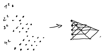
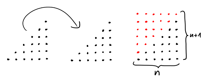
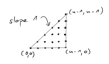
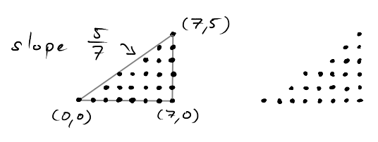
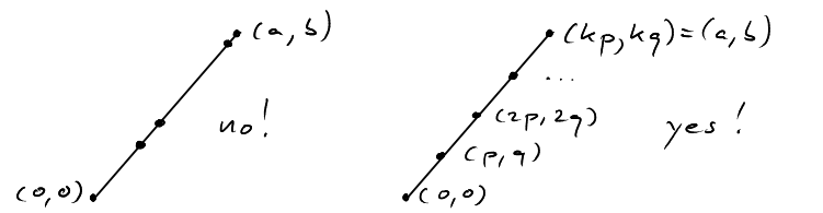
We have seen last time, that the sum \(\sum_{i=1}^n i\) counts the number of lattice points in triangles with slope 1. What geometric object is associated with \[\sum_{i=1}^n i^2?\]

\(\sum_{i=1}^n i^2\) counts the number of lattice points in pyramids.

Using this insight it is possible to derive the formula \[\sum_{i=1}^n i^2=\frac{n(n+2)(2n+1)}{6}.\]

We will not do that right now, but instead consider pyramids "with rational slope".

Pyramids

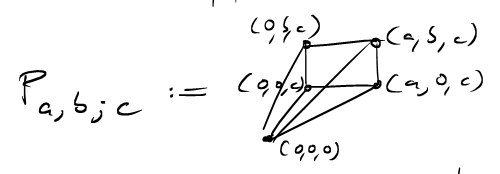
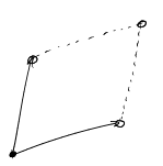
Notice that by reflection \(P_{a,b;c}=P_{b,a;c}\), which means that these pyramids are symmetric in the first two arguments but not in the last. Now, how many lattice points are in \(P_{a,b;c}?\) To this end, let us intersect the pyramid with a hyperplane, where the last coordinate is fixed.

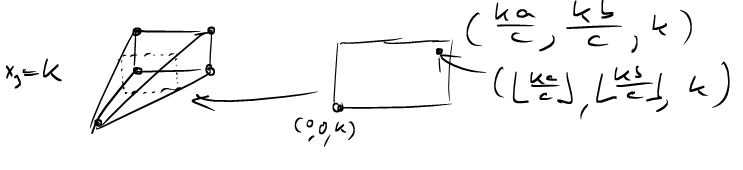
The top-right lattice point in each slice has coordinates \((\lfloor \frac{ka}{c} \rfloor, \lfloor \frac{kb}{c} \rfloor, k)\) and so the pyramid contains \[L(P_{a,b;c})= \sum_{k=0}^c (\left\lfloor \frac{ka}{c} \right\rfloor + 1) (\left\lfloor \frac{kb}{c} \right\rfloor + 1)\] lattice points.

In this sum, the "\(+1\)s" are kind of annoying, so can we modify the pyramids so that the lattice point count is exactly \(\sum_{k=0}^{c-1} \left\lfloor \frac{ka}{c} \right\rfloor \cdot \left\lfloor \frac{kb}{c} \right\rfloor\)?

One solution is to remove the hyperplanes given by \(x_1=0\), \(x_2=0\) and \(x-3=c\) from the pyramid. If \(\hat{P}_{a,b;c}\) is the "half-open" pyramid obtained by removing these hyperplanes from \(P_{a,b;c}\), then we have effectively removed one column and one row of lattice points from each "slice" and so, indeed, \[L(\hat{P}_{a,b;c}) = \sum_{k=0}^{c-1} \left\lfloor \frac{ka}{c} \right\rfloor \cdot \left\lfloor \frac{kb}{c} \right\rfloor.\]

Now, let’s try to do the same trick we did last time:

Can we build a simple geometric shape out of pyramids of this type in order to obtain a formula for these sums?

When last time, we built a rectangle out of triangles, this time, we are going to build a right-rectangular prism out of pyramids! (By the way, right-rectangular prims are called quader in German, which is a much shorter word, so I am going to stick to that one.) The idea is this:

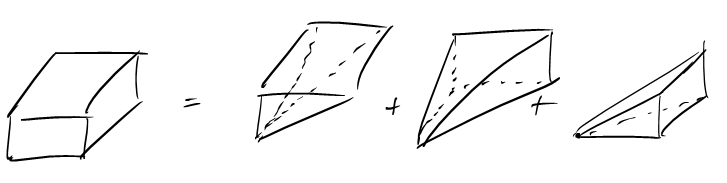
Let us consider the easy case first, where \(a,b,c\) are pairwise relatively prime, that is, \[\text{gcd}(a,b)=\text{gcd}(b,c)=\text{gcd}(a,c)=1.\]

How many lattice points are now on the triangles where two of the pyramids intersect?

In the relatively prime case, the only lattice points on this triangle are the origin and those on the line from \((0,b,c)\) to \((a,b,c)\). But all of these lie on hyperplanes that have been removed from our half-open pyramids! So the intersection of any two half-open pyramids does not contain any lattice points!

This means that in the relatively prime case, we will not have any double counting. Putting the three half-open pyramids together, we obtain the open quader \[\hat{P}_{a,b;c} \cup \hat{P}_{a,c;b} \cup \hat{P}_{b,c;a} = (0,a) \times (0,b) \times (0,c)\] where the union is disjoint, and so we get the formula \[L(\hat{P}_{a,b;c}) + L(\hat{P}_{a,c;b}) + L(\hat{P}_{b,c;a}) = L((0,a) \times (0,b) \times (0,c))\] which yields \[ \sum_{k=0}^{c-1} \left\lfloor \frac{ka}{c} \right\rfloor \cdot \left\lfloor \frac{kb}{c} \right\rfloor + \sum_{k=0}^{b-1} \left\lfloor \frac{ka}{b} \right\rfloor \cdot \left\lfloor \frac{kc}{b} \right\rfloor + \sum_{k=0}^{a-1} \left\lfloor \frac{kb}{a} \right\rfloor \cdot \left\lfloor \frac{kc}{a} \right\rfloor = (a-1)(b-1)(c-1).\]

This is a typical example of a reciprocity theorem. This term stems from the fact that fractions in which numerator and denominator have been exchanged are related, but I would like to use the term for a much wider class of theorems:

A reciprocity theorem is a theorem that puts several complicated functions (that, individually, have no simple form) in a simple relation.

We have been dealing with number theoretic functions here, but reciprocity theorems also exist for combinatorial counting functions, as we will see in a couple of weeks. In both cases, the message is that geometry helps finding reciprocity theorems.

Dedekind sums

Before we deal with the case where \(a,b,c\) are not relatively prime, let us first take a closer look at the sums \(\sum_{k=0}^{c-1} \left\lfloor \frac{ka}{c} \right\rfloor \cdot \left\lfloor \frac{kb}{c} \right\rfloor\). As it turns out these are closely related to so called Dedekind sums, which are important players in number theory.

The Dedekind sum \(s(a,b)\) is defined by \[s(a,b)=\sum_{k=0}^{b-1} \left(\left( \frac{ka}{b} \right)\right) \left(\left( \frac{k}{b} \right)\right)\] where \(((x))\) is the sawtooth function which is \(0\) if \(x\in\mathbb{Z}\) and \(\{x\}-\frac{1}{2}\) otherwise, where \(\{x\} = x - \lfloor x \rfloor\) is the fractional part of \(x\).

Dedekind sums are called Dedekind sums because of Dedekind’s reciprocity law which states that if \(\text{gcd}(a,b)=1\) then \[s(a,b)+s(b,a) = \frac{1}{12} \left( \frac{a}{b} + \frac{b}{a} + \frac{1}{ab} \right) - \frac{1}{4}.\]

Now, the first time I encountered Dedekind sums, I was baffled, because I had no idea what on earth this function was doing. Okay, Dedekind sums are periodic in the sense that \(s(a+b,b)=s(a,b)\) and this explains why they show up in the context of discrete Fourier transformation: Fourier transformation is a tool for the analysis of periodic functions, and Dedekind are the basic building blocks for this class of functions. But this does not answer the question:

What do Dedekind sums count or measure?

First of all, we notice that if \(\text{gcd}(a,b)=1\) the case that \(((x))=0\) if \(x\in\mathbb{Z}\) is never used: all arguments passed to the sawtooth function are fractional. This allows us to rewrite \(s(a,b)\) without the sawtooth function, using only fractional parts:

\[s(a,b) = \sum_{k=0}^{b-1} \left\{\frac{ka}{b}\right\}\left\{\frac{k}{b}\right\} - \frac{b}{2} + \frac{3}{4}\]

Given that \(\{x\}\) and \(\lfloor x \rfloor\) are complementary, you will not be surprised to hear that $_{k=0}^{b-1} \{\}\{\} $ and \(\sum_{k=0}^{c-1} \left\lfloor \frac{ka}{c} \right\rfloor \cdot \left\lfloor \frac{kb}{c} \right\rfloor\) are closely related. Can we see this relation in our pyramid picture?

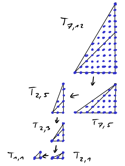
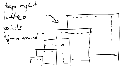
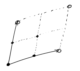
Let’s look at all the slices of the \(x_3=k\) hyperplanes with our pyramid. The complexity of the set of lattice points in this pyramid is tied to the fact that the top left lattice point in each slice appears "to jump around wildly". While the corners \((\frac{ka}{c},\frac{kb}{c},k)\) of the slices all lie on a line, the lattice points \((\lfloor \frac{ka}{c} \rfloor, \lfloor \frac{kb}{c} \rfloor, k)\) don’t.

This leads us to the following observation:

The sums \[s'(a,b;c) := \sum_{k=0}^{c-1} \left\{\frac{ka}{c}\right\}\left\{\frac{kb}{c}\right\}\] measure nothing but the area of the small rectangle between \((\lfloor \frac{ka}{c} \rfloor, \lfloor \frac{kb}{c} \rfloor, k)\) and \((\frac{ka}{c},\frac{kb}{c},k)\).

Before we look at a few examples, a short remark on the fractional-part function:

Decomposing a fraction \(\frac{a}{b}\) into its integral and fractional part \[\frac{a}{b} = \left\lfloor \frac{a}{b} \right\rfloor + \left\{ \frac{a}{b} \right\}\] amounts to the same thing as diving \(a\) by \(b\) with remainder: \[a = (a \text{ div } b)\cdot b +(a \text{ mod } b).\]

This gives us \[\left\lfloor\frac{a}{b} \right\rfloor = a \text{ div } b \;\;\;\text{ and }\;\;\; \left\{ \frac{a}{b} \right\} = \frac{a \text{ mod } b}{b}.\]

Of course this is just notation. But to me, it serves as a reminder that we are doing just modular arithmetic here and not dealing with "real" real numbers. Also, we get \[ s'(a,b;c) = \frac{1}{c^2} \sum_{k=0}^{c-1} (ka \text{ mod }c)\cdot(kb\text{ mod } c)\] and can read off that \(c^2\cdot s'(a,b;c)\) is integral - so it counts something!

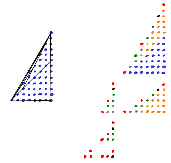
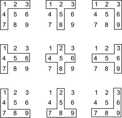
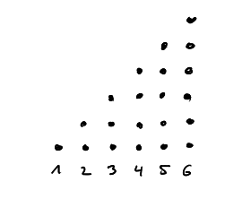
Let us now visualize \(c^2\cdot s'(a,b;c)\) by drawing the "rectangles" \((ka \text{ mod }c)\cdot(kb\text{ mod } c)\) for \(k=0,\ldots,c-1\). We pick the example \[7^2\cdot s'(5,1;7) = 5\cdot 1 + 3 \cdot 2 + 1 \cdot 3 + 6 \cdot 4 + 4 \cdot 5 + 2 \cdot 6.\]

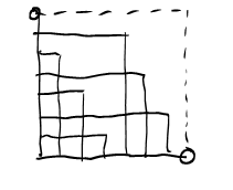
How does the "corner" defining the rectangle move when we pass from one column \(k\) to the next? As we are doing modular arithmetic here, we are operating on a torus here. We can see this by identifying the top and bottom, and left and right edges of this square, respectively. Moving from one corner to the next corresponds to translation by the vector \((5,1)\) on the torus. So the corners of these rectangles all lie on one line.

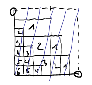
In the above image, each region is labled with a number. This number gives the number of rectangles this region is contained in. If we now consider all sums \(s'(a,1;7)\) for \(a=1,\ldots,6\) we get all (linear) lines \(\text{mod }7\).

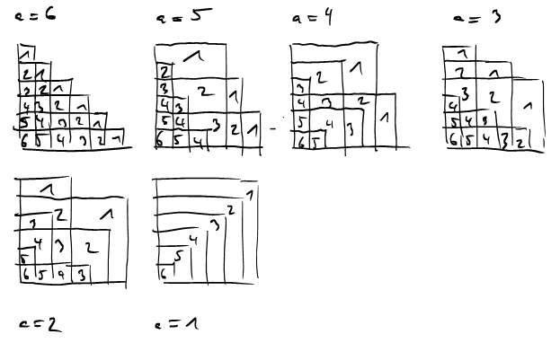
Note that in the relatively prime case it suffices to consider sums of the form \(s'(a,1;c)\) because \[s'(a,b;c) = s'(ab^{-1},1;c)\] where \(b^{-1}\) denotes the multiplicative inverse of \(b\) modulo \(c\). Can you see this in the picture?

Now, here are two questions for you:

Question. Does this visualization give an immediate geometric proof of Dedekind reciprocity? Why do \(s'(a,1;b)\) and \(s'(b,1;a)\) sum to something simple?

Question. We have proved a reciprocity law for the "pyramid sums" \(L(\hat{P}_{a,b;c})\). Is this reciprocity law equivalent to some classic reciprocity law for Dedekind sums and their generalizations?

For inspiration in this regard, you may want to consult Chapter 8 of Computing the Continuous Discretely by Matthias Beck and Sinai Robins.

Pyramids with Lattice Points on the Boundary

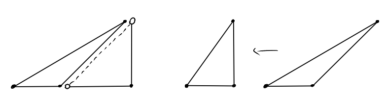
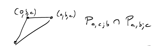
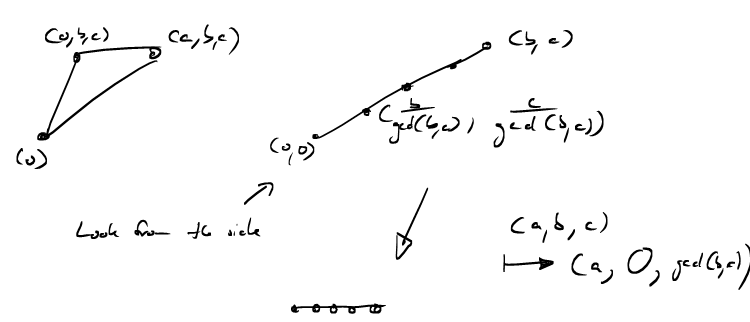
I promised to work out the reciprocity law for \(L(\hat{P}_{a,b;c})\) when \(a,b,c\) are not relatively prime. To this end we need to work out the number of lattice points in the triangle \[P_{a,b;c} \cap P_{a,c;b} =\text{conv}( \;(0,0,0), \; (0,b,c) ,\; (a,b,c) \; ).\]

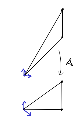
We want to find a lattice transformation that maps this triangle into one of our coordinate hyperplanes, so that we can apply last lecture’s formula for counting lattice points. Let’s look at this triangle from the side, along the \(x_1\)-axis. Then it looks just like a line from \((0,0,0)\) to \((0,b,c)\). This line contains \(\text{gcd}(b,c)+1\) lattice points. The "first" lattice point after the origin has coordiantes \((0,\frac{b}{\text{gcd}(b,c)},\frac{c}{\text{gcd}(b,c)})\). We would now like to map this line onto the (in this picture) horizontal axis, such that \((0,b,c)\) is mapped to \((0,0,\text{gcd}(a,b))\), so that the \(\text{gcd}(b,c)+1\) lattice points on the line are mapped to \(\text{gcd}(b,c)+1\) adjacent lattice points on the \(x_3\)-axis. We do not want to affect the \(x_1\)-coordinate at all, so we, similarly, want to map \((a,b,c)\) to \((a,0,\text{gcd}(b,c))\).

Let’s work out the matrix for this lattice transformation. We want \[\begin{pmatrix} ? & ? & ? \\ ? & ? & ? \\ ? & ? & ? \end{pmatrix} \cdot \begin{pmatrix} a \\ b \\ c \end{pmatrix} = \begin{pmatrix} a \\ 0 \\ \text{gcd}(b,c) \end{pmatrix}.\]

As the first coordinate is supposed to remain invariant, we put \[\begin{pmatrix} 1 & 0 & 0 \\ 0 & ? & ? \\ 0 & ? & ? \end{pmatrix} \cdot \begin{pmatrix} a \\ b \\ c \end{pmatrix} = \begin{pmatrix} a \\ 0 \\ \text{gcd}(b,c) \end{pmatrix}.\]

How can we combine \(b\) and \(c\) to get \(\text{gcd}(b,c)\)? This is precisely what the extended Euclidean algorithm does for us. It computes integers \(x\) and \(y\) such that \(xb+yc=\text{gcd}(b,c)\) which gives us \[\begin{pmatrix} 1 & 0 & 0 \\ 0 & ? & ? \\ 0 & x & y \end{pmatrix} \cdot \begin{pmatrix} a \\ b \\ c \end{pmatrix} = \begin{pmatrix} a \\ 0 \\ \text{gcd}(b,c) \end{pmatrix}.\]

Now we want to fill in the second row such that \(b\) and \(c\) cancel out. A good first idea is \[\begin{pmatrix} 1 & 0 & 0 \\ 0 & -c & b \\ 0 & x & y \end{pmatrix} \cdot \begin{pmatrix} a \\ b \\ c \end{pmatrix} = \begin{pmatrix} a \\ 0 \\ \text{gcd}(b,c) \end{pmatrix}.\]

But this matrix does not have all the properties we would like. We also want it to be a lattice transform, so in particular, its determinant has to be \(\pm 1\). Currently, however, the determinant is \[-cy-bx=-\text{gcd}(b,c).\] So what we have to do is divide those two entries by \(\text{gcd}(b,c)\) to give us our final matrix:

\[\begin{pmatrix} 1 & 0 & 0 \\ 0 & -\frac{c}{\text{gcd}(b,c)} & \frac{b}{\text{gcd}(b,c)} \\ 0 & x & y \end{pmatrix} \cdot \begin{pmatrix} a \\ b \\ c \end{pmatrix} = \begin{pmatrix} a \\ 0 \\ \text{gcd}(b,c) \end{pmatrix}.\]

This is a lattice transform and it maps

\[\begin{pmatrix} 1 & 0 & 0 \\ 0 & -\frac{c}{\text{gcd}(b,c)} & \frac{b}{\text{gcd}(b,c)} \\ 0 & x & y \end{pmatrix} \cdot \begin{pmatrix} 0 \\ \frac{b}{\text{gcd}(b,c)} \\ \frac{c}{\text{gcd}(b,c)} \end{pmatrix} = \begin{pmatrix} 0 \\ 0 \\ 1 \end{pmatrix}\]

and

\[\begin{pmatrix} 1 & 0 & 0 \\ 0 & -\frac{c}{\text{gcd}(b,c)} & \frac{b}{\text{gcd}(b,c)} \\ 0 & x & y \end{pmatrix} \cdot \begin{pmatrix} 0 \\ -y \\ x \end{pmatrix} = \begin{pmatrix} 0 \\ 1 \\ 0 \end{pmatrix}.\]

So the lattice point \((0,-y,x)\) corresponds to the standard unit vector \((0,1,0)\) in this bijection. Can we interpret this somehow?

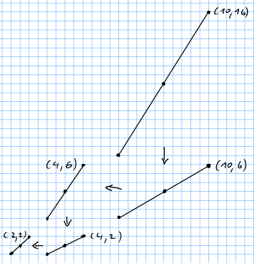
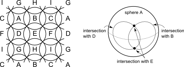
Let’s look at an example. Let \(b=10\) and \(c=14\) such that \(\text{gcd}(b,c)=2\). Then \[ 3 \cdot 10 - 2 \cdot 14 = 2 \] so $x= 3 $ and \(y=-2\) and the mysterious lattice point is \((0,2,3)\).

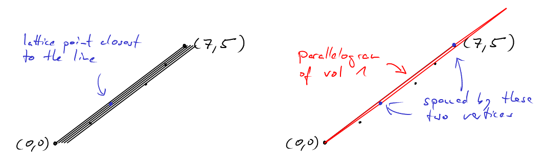
In this picture there are two things to notice:

1. Consider all translates of the line through \((0,0)\) and \((10,14)\) that go through some lattice point. \((2,3)\) lies on the translate closest to the original.
2. The vectors \((2,3)\) and \((5,7)\) span a parallelogram of volume 1.

These are no accidents. \((2,3)\) and \((5,7)\) form a lattice basis. And the task of finding a lattice transformation to the standard basis is equivalent to finding a lattice basis. Let us make these notions precise.

Lattice Bases

Recall that a lattice transformation \(f:\mathbb{R}^d\rightarrow\mathbb{R}^d\) is an affine isomorphism that, when restricted to the integer lattice \(\mathbb{Z}^d\), induces a bijection (i.e., a 1-to-1 and onto map) on the integer lattice \(f|_{\mathbb{Z}^d}: {\mathbb{Z}^d} \rightarrow {\mathbb{Z}^d}\). Now, a lattice basis is a set \(a_1,\ldots,a_d\in\mathbb{Z}^d\) of linearly independent integer vectors such that for every \(z\in\mathbb{Z}^d\) there exist integers \(\lambda_1,\ldots,\lambda_d\in\mathbb{Z}\) such that \[\sum_{i=1}^d \lambda_i a_i = z.\]

These notions are closely related. For linearly independent integer vectors \(a_1,\ldots,a_d\in\mathbb{Z}^d\) the following are equivalent:

• \(a_1,\ldots,a_d\) form a lattice basis.
• There exists a lattice transformation \(f\) such that \(f(a_i)=e_i\) for \(i=1,\ldots,d\) where \(e_i\) are the standard unit vectors.
• The fundamental parallelepiped \(\Pi_{a_1,\ldots,a_d}\) contains exactly one lattice point \(z\in\mathbb{Z}^d\)

Here, the fundamental parallelepiped \(\Pi_{a_1,\ldots,a_d}\) spanned by \(a_1,\ldots,a_d\) is the set

The crucial ingredient to the proof of the above equivalences is the following theorem.

Theorem. Let \(a_1,\ldots,a_d\in\mathbb{Z}^d\) be linearly independent integer vectors. Let \(A=(a_1 \; \ldots \;a_d)\) be the matrix with the \(a_i\) as columns. Then \[L(\Pi_{a_1,\ldots,a_d}) = \text{Volume}(\Pi_{a_1,\ldots,a_d}) = |\det(A)|.\]

Now, as we will see, it is always the case that the lattice point count approximates the volume in a certain sense. But for fundamental parallelepipeds we have equality here! The reason is the following.

Sketch of Proof. First of all we make the approximation argument a bit more precise, by arguing that

\[\lim_{k\rightarrow\infty} \frac{1}{2^{kd}}|\frac{1}{2^k}\mathbb{Z}^d \cap \Pi_{a_1,\ldots,a_d}| = Volume(\Pi_{a_1,\ldots,a_d}).\]

Instead of counting lattice points in some set \(X\), we can also measure the volume of a set of unit cubes, that each have one of these lattice points at their center. Intuitively, this is a rough approximation of the volume of the set.

Next, we refine this approximation in the following way. We refine the lattice \(\mathbb{Z}^d\) by scaling it by \(\frac{1}{2}\). Now we play the same game with the cubes, measuring the volume of a set of cubes, each with one of the lattice points in \(X\) at its center. To make sure that the cubes don’t overlap we have to scale their sidelengths by \(\frac{1}{2}\) as well, which scales their volume by \(\frac{1}{2^d}\).

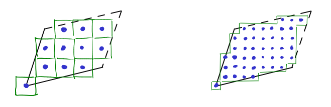
If we continue in this fashion, we our cube set in the \(k\)th step will have volume \(\frac{1}{2^{kd}}|\frac{1}{2^k}\mathbb{Z}^d \cap \Pi_{a_1,\ldots,a_d}|\). And we can see that the volume of this cube set approximates the volume of the parallelepiped, in the same way that the number of pixels, multiplied by the area of a pixel, will approximate the area of a parallelogram drawn on a (very high resolution) computer screen.

So far, this works for all polytopes, not just for the parallelepiped. But now comes the curcial property of the fundamental parallelepiped.

\[ L(k\cdot\Pi_{a_1,\ldots,a_d}) = k^d \cdot L(\Pi_{a_1,\ldots,a_d}) \]

The reason is simply that we can tile the \(k\)-th dilate of \(\Pi_{a_1,\ldots,a_d}\) by \(k^d\) integral translates of \(\Pi_{a_1,\ldots,a_d}\). Because these are integral translates, they all contain the same number of lattice points as the original fundamental parallelepiped.

Now all we have to observe is that refining the lattice is the same as dilating our parallelepiped. Then, our proof is simply this:

\[ L(\Pi_{a_1,\ldots,a_d}) =\lim_{k\rightarrow\infty} \frac{1}{2^{kd}} L(2^k\cdot \Pi_{a_1,\ldots,a_d}) = \lim_{k\rightarrow\infty} \frac{1}{2^{kd}} |\frac{1}{2^k}\mathbb{Z}^d \cap \Pi_{a_1,\ldots,a_d}| = \text{Volume}(\Pi_{a_1,\ldots,a_d}).\]

Conclusion

After this detour, let us finally put our reciprocity theorem in the non-relatively prime case together.

Using our lattice transformation, we have seen that \[L(\text{conv}( \;(0,0,0), \; (0,b,c) ,\; (a,b,c) \; )) = L(\text{conv}( \;(0,0,0), \; (0,0,\text{gcd}(b,c)) ,\; (a,0,\text{gcd}(b,c)) \; ))\]

Using our formula from the last lecture, we conclude that

\[L(\text{conv}( \;(0,0,0), \; (0,0,\text{gcd}(b,c)) ,\; (a,0,\text{gcd}(b,c)) \; )) = \frac{(a+1)\text{gcd}(b,c) + \text{gcd}(a,b,c) + 1}{2}\]

We now have to adjust for the fact that the pyramids \(\hat{P}_{a,b;c}\) are half open. In particular, the two "rectangular" sides have been removed (when intersecting half open pyramids). This gives us

\[ L(\hat{P}_{a,b;c}\cap \hat{P}_{a,c;b}) = \frac{(a+1)\text{gcd}(b,c) + \text{gcd}(a,b,c) + 1}{2} - a - \text{gcd}(b,c) - 1\]

which simplifies to

\[ L(\hat{P}_{a,b;c}\cap \hat{P}_{a,c;b}) = \frac{1}{2}\left((\text{gcd}(b,c) -2) a - \text{gcd}(b,c) + \text{gcd}(a,b,c) -1\right).\]

These observations also allow us to compute the number of lattice points on the diagonal

\[ L(\hat{P}_{a,b;c}\cap \hat{P}_{a,c;b} \cap \hat{P}_{b,c;a}) = \text{gcd}(a,b,c) -1. \]

Now we can out all of these formulas together by applying inclusion-exclusion.

\[ \begin{eqnarray} (a-1)(b-1)(c-1) & = & L(\hat{P}_{a,b;c}) + L(\hat{P}_{a,c;b}) + L(\hat{P}_{b,c;a}) \\ && - L(\hat{P}_{a,b;c}\cap \hat{P}_{a,c;b}) - L(\hat{P}_{a,b;c}\cap \hat{P}_{b,c;a}) - L(\hat{P}_{a,c;b}\cap \hat{P}_{b,c;a}) \\ && + L(\hat{P}_{a,b;c}\cap \hat{P}_{a,c;b} \cap \hat{P}_{b,c;a}) \end{eqnarray} \]

This yields

And all of this, just because we fit three pyramids together to form a quader!

While the first two lectures focused on two examples of how visualizing numbers can yield actual formulas, we are going to start with some theory in the next lecture and talk about polytopes. So you do not have to worry: the next lecture is not about \(\sum_k k^3\)! Here is another question, though:

Can you work out the classic formula for \(\sum_k k^d\) by putting \(d\) pyramids over a \(d-1\) cube together?

Gauss’ sum formula

One of mathematic’s most well-known anecdotes tells a story about Carl Friedrich Gauss when he was still a boy. At the Volksschule in Braunschweig, his math teacher gave the class the assignment of summing all integers from 1 through 100, with the intent of keeping them busy for a while. But as soon as the teacher had posed this problem, young Gauss wrote down his answer and shouted: "There it is!" To everyone’s astonishment he had written down the correct number: 5050.

What had happend was that Gauss had refused to churn numbers, the way his teacher had intended him to. Instead he had done mathematics! He had come up with the formula \[\sum_{i=1}^{n} i = \frac{n(n+1)}{2}\] and applied it to the case \(n=100\) to get his result.

This formula was known at the time - but not to Gauss. So the natural question is to ask, how Gauss had come up with this formula. Proving this formula may be a routine exercise. But where had his idea come from that something like this might hold?

Of course, I do not know what went on in Gauss’ head and I certainly agree that Gauss was one of the greatest mathematicians of all times. But what I would like to argue here is this:

It does not take a genius to come up with formula. All it takes is some intuition about numbers.

Here I would like to describe one such intuition that leads to this formula.

We visualize the number \(i\) simply as a set of \(i\) points. For convenience we place all these points in one column. Taking the sum now simply means taking the disjoint union of these sets of points. In case of the sum \(\sum_{i=1}^n i\) this yields a triangle of points.

Now, we have no idea (yet) how to count point in triangles. But we have a very good idea of how to count points in rectangles: that’s just what multiplication is for! So we take two instances of this triangle and fit them together such that they form a rectangle of \(n\) by \(n+1\) points.

This shows \[2\cdot \sum_{i=1}^n i = n(n+1)\] which implies Gauss’ formula.

Note: A video in which I tell just this story in German can be found here.

Lattice Points in Triangles

Crucial to the above argument was that we arranged the points in a regular pattern. In fact, we used points \(x\) in the lattice \(\mathbb{Z}^2\). Throughout these lectures a lattice point or integer point will be an element of the integer lattice \(\mathbb{Z}^n\) for some \(n\). There are other lattices, but we will only work with this one. For convenience, we will write \(L(X)= |\mathbb{Z}^n\cap X|\) for the number of lattice points in some set \(X\subset\mathbb{R}^n\).

In the above proof, we used the set of lattice points contained in the triangle

The two "instances" of this triangle fit together so nicely, because the line \(x_1=x_2\) corresponding to the inequality \(x_1\geq x_2\) has slope 1. Thus, whenever we move one column to the right, the number of lattice points in the column always changes by one. What happens when we consider triangles with more general (rational) slopes?

Let \(T_{a,b}\) denote the triangle with slope \(\frac{b}{a}\) for \(a,b\in\mathbb{N}\).

Here, the "steps" we take from one column to the next become irregular. Sometimes we go one lattice point up, sometimes we don’t. But before we take another look at the structure of this lattice point set, let us simply count how many lattice points there are.

Counting Lattice Points

Counting the number of lattice points in \(T_{a,b}\) is easy enough.

\[ L(T_{a,b}) = |\mathbb{Z}^2 \cap T_{a,b}| = \sum_{k=0}^a \left( \left\lfloor \frac{kb}{a} \right\rfloor + 1 \right)\]

But what we really want is a simple expression for the sum on the right hand side. Let us try a variation of the previous trick to find one!

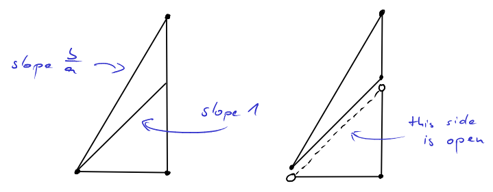
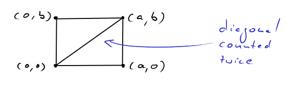
We can fit two "instances" of the triangle \(T_{a,b}\) together to form the rectangle \(R=[0,a]\times[0,b]\). All lattice points in \(R\) are contained in exactly one of the two triangles, except for the lattice points on the diagonal

The lattice points on the diagonal \(D\) are contained in both triangles and are thus counted twice in the following sum.

So how many lattice points are on the diagonal?

Lemma. The number of lattice points on the diagonal \(D_{a,b}\) is the greatest common divisor of \(a\) and \(b\) plus one, that is, \[L(D_{a,b}) = \text{gcd}(a,b) +1.\]

Proof. We make the following observations.

1. The lattice points on the diagonal parition the diagonal into intervals of equal length.

This follows simply from the fact that the difference between to lattice points is an integer vector and translation by an integer vector maps lattice points to lattice points.

2. Let \((p,q)\in D\cap\mathbb{Z}^2\) such that \(p>0\) is minimal. Let \(k\) be the number of intervals into which \(D\) is partitioned. Then \[kp = a \;\;\; \text{and} \;\;\; kq = b.\] So \(k\) is a common divisor of \(a\) and \(b\).

3. Conversely, let \(k'\) be a common divisor of \(a\) and \(b\). This means, there exist \(p',q'\in \mathbb{Z}^2\) such that \[ k'p' = a \;\;\; \text{and} \;\;\; k'q' = b,\] which implies \(\begin{pmatrix} p \\ q\end{pmatrix}=\frac{1}{k'}\begin{pmatrix} a \\ b\end{pmatrix},\) which in turn means that \((p',q')\) is a lattice point on the diagonal \(D_{a,b}\).

As \(p\) was chosen minimal, we conclude that \(p' \geq p\) and thus \(k' \leq k\), which means that \(k\) is the greatest common divisor of \(a\) and \(b\). The number of lattice points on the diagonal is \(k+1\). QED.

Great! Now we have both: a visual interpretation of the \(\text{gcd}\) and the means to complete our formula!

\[\sum_{k=0}^a \left( \left\lfloor \frac{kb}{a} \right\rfloor + 1 \right) = \frac{(a+1)(b+1) + \text{gcd}(a,b) + 1}{2}\]

Note that by symmetry we also get

\[\sum_{k=0}^b \left( \left\lfloor \frac{ka}{b} \right\rfloor + 1 \right) = \frac{(a+1)(b+1) + \text{gcd}(a,b) + 1}{2}.\]

This corresponds to the fact that the lattice point sets in \(T_{a,b}\) and \(T_{b,a}\) are "the same". Let us make this notion precise.

Lattice Isomorphism

We want to answer questions such as "How many lattice points are in a set \(S\)?" From this point of view, we want to see two sets as "the same" when there is a linear automorphism from the ambient space to itself that induces a bijection on the lattice. Then, applying the automorphism does not changes the number of lattice points in any given set.

So, a lattice isomorphism is an affine linear map \(f:\mathbb{R}^n\rightarrow\mathbb{R}^n\) of the form \(f(x)=Ax+b\) that induces a bijection from \(\mathbb{Z}^n\) onto itself. We say set \(X\) is a lattice transform of a set \(Y\) if there exists a lattice isomorphism \(f\) with \(f(X)=Y\).

Lattice isomorphisms are very useful objects. We have already made implicit use of the fact that translations by an integer vector and reflections at the origin are lattice isomorphisms. And our observation that \(T_{a,b}\) and \(T_{b,a}\) have "the same" lattice point structure can be made precise by saying that

is a lattice isomorphism.

We will need one more lattice isomorphism in a minute. And to show that it is a lattice isomorphism, we will make use of the following tool.

Lemma. The map \(x\mapsto Ax +b\) is a lattice isomorphism if and only if \(A\) and \(b\) are integral and \(\det(A) = \pm 1\).

The proof is not difficult, and we omit it for now.

Structure of \(\mathbb{Z}^2\cap T_{a,b}\)

We now know how many lattice points there are in \(T_{a,b}\). But what we would really like to understand is the structure of this set of lattice point. When we look at larger examples of these triangles than we see that this "staircase" of points appears "irregular" but far from "random". What is going on here?

One way to approach this question is by investigating the recursive structure of these lattice point sets. We can ask:

What subset of \(\mathbb{Z}^2\cap T_{a,b}\) is particularly easy to describe?

As we have seen in the example of Gauss’ sum formula, triangles with integral slopes are particularly easy to describe.

Let us suppose that \(a < b\). This means that the slope \(\frac{b}{a}\) of the triangle is "steep". In this case, we can find a subset of the lattice points which corresponds to a triangle with integral slope. Or, more precisely, \[\mathbb{Z}^2\cap T_{a,a} \subset \mathbb{Z}^2\cap T_{a,b}.\]

Let us split the triangle \(T_{a,b}\) into two parts. A lower part with integral slope that is easy to describe and an upper part that we have yet to make sense of. Both parts meet at the line \(x_1=x_2\). For convenience, we decide that this boundary should belong to the upper part and it should be removed from the lower part. The lower part then becomes a half-open triangle of the form

In this way we can partition \(T_{a,b}\) such that

the lower part \(\mathbb{Z}^2\cap T'_{a,a}\) has a simple form and precisely \(\frac{a(a+1)}{2}\) lattice points.

Good. What about the upper part \(T_{a,b}\setminus T'_{a,a}\)?

We would like to see that this upper part is again a triangle of the form we have been studying all the time, so that we apply recursion. To that end we need to transform the upper part so as to create a right angle at the vertex on the bottom-right. To achieve this we might try to shear the triangle. But is the resulting linear transformation a lattice isomorphism?

As we can see the matrix of the linear transformation is simply

As \(\det(A)=1\) we conclude that this transformation is a lattice isomorphism and thus:

The upper part \(T_{a,b}\setminus T'_{a,a}\) is a lattice transform of \(T_{a,b-a}\).

So we can simplify "steep" triangles until we obtain a "flat" triangle with slope \(<1\). But by our observation that

\(T_{a,b}\) is a lattice transform of \(T_{b,a}\)

we can turn "flat" triangles into "steep" triangles and continue with this method of simplification! Equivalently, we can handle flat triangles by partitioning them differently and shearing "left" instead of "down".

We have thus obtained a recursive description of the sets of lattice points in the triangles \(T_{a,b}\).

This allows us to decompose the set of lattice points in a large triangle \(T_{a,b}\) into lattice transforms of "simple" sets of lattice points.

(Note: There are other ways of making sense of this "staircase" of lattice points. If you got curious, I would like to advertise Fred’s and my article on "Staircases in \(\mathbb{Z}^2\)".)

As a side-effect, this recursion also allows us to count the lattice points in \(T_{a,b}\) recursively.

Theorem. Let \(a,b\in\mathbb{N}\). Then:

1. If \(a>b\) then \(L(T_{a,b})=L(T_{a-b,b}) + \frac{b(b+1)}{2}\).
2. If \(a < b\) then \(L(T_{a,b})=L(T_{a,b-a}) + \frac{a(a+1)}{2}\).
3. \(L(T_{a,a})=\frac{(a+1)(a+2)}{2}\).

Apart from the structural insight, what does the recursion for \(L(T_{a,b})\) buy us? With \[L(T_{a,b})=\frac{(a+1)(b+1) + \text{gcd}(a,b) + 1}{2}\] we already have a very nice closed form expression for \(L(T_{a,b})\), don’t we?

Well, not quite. \(\text{gcd}(a,b)\) is no closed form expression. To compute \(\text{gcd}(a,b)\) we need to use the Euclidean Algorithm. In fact, I would like to argue that the above recursion is essentially the same as the Euclidean Algorithm.

Visualizing the Euclidean Algorithm

I would like to close this lecture by arguing that the recursion we developed in the previous section is nothing but a visualization of the Euclidean Algorithm. A simple description of the Euclidean Algorithm (which he called "antenaresis") is this:

"[The greatest common divisor] can be found using antenaresis by repeatedly subtracting the smaller, whichever it happens to be at the time, from the larger until the smaller divides the larger." Euclid’s Elements

When we apply the above recursion to compute \(L(T_{a,b})\), we do exactly the same thing, as far as the pair \((a,b)\) is concerned! If \(a>b\) we pass to \((a-b,b)\) and if \(a < b\) we pass to \((a,b-a)\). Even the stopping criteria are essentially the same, even though they look different at first glance.

So here is a "geometric interpretation" of the Euclidean Algorithm:

1. We want to compute the greatest common divisor of \(a\) and \(b\). As we have seen this amounts to computing the number of lattice points on the diagonal \(D_{a,b}\) of the rectangle \([0,a]\times[0,b]\).
2. To achieve this, we apply lattice transformations. These do not change the number of lattice points on the diagonal.

• If \(a > b\) we shear the diagonal "left" and pass to \(D_{a-b,b}\).
• If \(a < b\) we shear the diagonal "down" and pass to \(D_{a,b-a}\).

3. We stop as soon as the number of lattice points on the diagonal can be read of immediately. For example, if we reach a line of the form \(D_{a,a}\) or \(D_{a,ka}\) or \(D_{a,0}\).

So in a way,

all the Euclidean Algorithm does is compressing a set of lattice points by means of lattice transformations!

For our two formulas for \(L(T_{a,b})\) this means that both use the same type of recursion. This of course begs the question:

Is there a faster way to compute the \(\text{gcd}\) of two integers? Is there maybe even a "closed form" expression for \(\text{gcd}\)?

As it turns out, these questions are closely related to a long standing open problem in complexity theory:

Is the problem of computing the \(\text{gcd}\) in the complexity class \(\mathbf{AC}\)?

Informally, this is asking whether there exists a family of boolean circuits with polynomial size, polylogarithmic-depth and unbounded fan-in that computes the \(\text{gcd}\). See the Complexity Zoo for more information.

Outlook

This is it for today! Next time, we will continue visualizing numbers and venture into the world of Dedekind sums.

This post is about different approaches to font rendering, what you can do if you prefer smooth over crisp fonts but are stuck on the Windows platform and how you can make sure Firefox and Qute take advantage of this workaround. But let’s start from the beginning…

Motivation: EPUB versus PDF

Several people have called my attention to the EPUB document format as an alternative to PDF. Ya Knygar asked about an EPUB export option for Qute. Peter discussed math support in EPUBs. And we had a chat about the topic with the nice people from Design Science.

All in all, I think the format has great promise and I will definitely add an EPUB export option to Qute as soon as I have time. But there is one reason why I am not going to switch from PDF to EPUB anytime soon (even if EPUBs were widely available): In my opinion,

PDF readers have superior text rendering compared to EPUB readers.

Now, you may think that this problem will go away soon as EPUB readers improve. But things are not so simple. In this post, I will explain what the problem is exactly, why it won’t go away soon, and what you can use as a workaround for the time being.

Before we start, I have to mention that the problem I am talking about affects only the Windows platform and mostly devices with low pixel density. It you are running Linux, you are probably fine, and if you are running Windows on your tablet, chances are good that the differences I am talking about are hardly noticeable. But if you are running Windows and plan to read PDF/EPUB articles on your desktop 23 inch Full HD screen, this might concern you.

Smooth versus crisp

The most important thing to understand about font rendering, is that there is no single “best” way to render a font. There are simply two different goals you might wish to achieve. You may want to:

1. Optimize the contrast of the font to increase readability.
2. Optimize the shape of the font to make it look pretty.

These objectives are in conflict with each other.

If accessibility is your primary objective, you want to optimize contrast. This means that you have to align the glyphs with the pixel grid of your screen. But if the font size is low, this means that you will have to distort the individual glyphs of the font. The result is crisp distorted text. This is the approach taken by Microsoft in their font rendering engines, including ClearType and DirectWrite.

If aesthetics are your primary objective, you want to optimize the shape of the font. That is, you want to reproduce the glyphs on screen exactly as the font designer intended. At low font sizes this is, of course, impossible. You will instead have to super-sample the individual glyphs and use lots of gray-scale pixels to give the illusion of an accurate shape. The result is smooth and accurate but blurry text. This is the approach taken by Apple in their font rendering engine, and, apparently, it is the approach taken by Adobe in the font rendering engine employed by the Adobe Acrobat PDF reader.

Now, we come to an example. The following text snippet is taken from Martin Fenner’s blog and typeset in Palatino Linotype. On the left it is reproduced in an EPUB document which is rendered by EPUBReader on Windows 7 while ClearType is turned on. On the right it is reproduced in a PDF document which is rendered by Adobe Acrobat Reader on Windows 7. (Note that these images may look different on your screen than they do on mine due to different subpixel orderings.)

Opinions about which rendering is better will differ. Personally, I think “smooth but blurry” is far better than “crisp but distorted”.

This is especially true of in case of serif fonts. There is no doubt that the ClearType approach can render sans serif fonts beautifully, e.g., Consolas as rendered on Windows 7. But with most serif fonts, trying to align them automatically with the pixel grid is simply a lost cause.

Technological Subtleties

If you experiment with viewing EPUBs in different applications, you will notice two things:

1. On platforms other than Windows EPUBReader renders EPUBs just fine.
2. All EPUB readers on Windows suffer from this font rendering problem (including Adobe’s Digital Editions).

These two phenomena have a common cause: EPUB readers typically use the layout engines of popular webbrowsers to display text. These layout engines, in turn, use the font rendering API of the operating system to render text.

These two facts will not change in the near future. The layout of HTML code is a complex task, so EPUB readers will rely on browsers to do the job for them. (This is also witnessed by the fact, that even though the Adobe Reader has an excellent font rendering system, Adobe Digital Editions does not use it. Even though Adobe can do font rendering better than the OS, they cannot do text layout better than web browsers.)

Browsers, in turn, will rely on OS font rendering mechanisms, in order to guaranty consistency of text rendering across all applications on a given system. In this regard, web browsers differ fundamentally from PDF viewers. Adobe Acrobat’s job is to render pages exactly the same on all platforms. For web browsers and for the EPUB format, this is a non-objective.

In many ways, this is a good thing! EPUB allows users to customize the appearence of a document to their liking, and I am all for that! The only downside is that if 1) I disagree with the font rendering algorithm of my operating system, and 2) I can’t switch operating systems until there comes a Linux for tablet PCs with decent digital ink support along, I am stuck.

Workaround: GDI++

As it turns out, I am not quite stuck. Thanks to GDI++.

GDI++ is a marvelous little library, that replaces the standard GDI font rendering mechanism on Windows with a font rendering mechanism based on FreeType. You can activate and deactivate GDI++ from a tray icon, and as easy as that, have all Windows applications have beautiful smooth FreeType-rendered fonts! On top of that GDI++ is highly configurable - even though I have to admit, that I have not tried all of these options yet.

Of course, there are some pitfalls.

First of all, GDI++ does not appear to be actively maintained. On this page, there is an announcement stating that GDI++ development has been discontinued. However, there are still a number of updates available here, some as recent as 2011. The wiki mentions InkStone as a follow-up project. But, apparently, InkStone development never got going.

Second, most of the GDI++ documentation as well as the community web pages are in Japanese. So, for me at least, it is quite hard to figure out what is going on. (Even though Google’s translation services are a big help.)

Third, GDI++ changes the font rendering only in those applications that use GDI for drawing text. This includes, for example, such heavyweights as Microsoft Word, which all of sudden becomes really pleasant to look at. (If I had know about GDI++ from the start, I might not have been driven to such as extremes as writing my own text editor…) But not all Windows applications use GDI.

Firefox and GDI++

Chrome works with GDI++ version 8.1.2009.0211 out of the box. But Firefox does not.

When you activate GDI++ from the tray, all text in Firefox (including the EPUBs rendered by EPUBReader) remain unaffected. The reason is that recent versions of Firefox use Direct2D as rendering engine and not GDI. The advantage of this approach is that web pages in Firefox are rendered using hardware acceleration! The drawback is that GDI++ does not work.

To get GDI++ to work with Firefox, you need to disable Firefox’ hardware acceleration. You can do this via the “Advanced Properties” tab, where you need to uncheck the “use hardware acceleration” box. After a restart while gditray is running, Firefox should render beautifully antialiased text.

The following example shows the aforementioned text snippet rendered by EPUBReader using ClearType/DirectWrite (on the left) and using FreeType/GDI++ (on the right).

To my eye, the FreeType version is so much better! The font now actually looks like Palatino!

The rendering is not perfect, however. A direct comparison of FreeType/GDI++ (left) with Adobe Acrobat Reader (right) is shown below. While the Adobe rendering is a bit too light for my taste, it is clearer than the FreeType rendering. A compromise between these two would be optimal, in my opinion.

On the whole, I definitely want to use GDI++ for EPUB reading. But whether I want to do all my browsing with Firefox’ hardware acceleration turned off is another matter. If hardware acceleration is a must, another option is to use Firefox’ Anti-Aliasing Tuner, which allows you to tweak the Direct2D font rendering. If you use the “Outline” rendering mode, you get results similar to FreeType/GDI++. However, even after quite some experimentation with the Anti-Aliasing Tuner’s options, I have not been able to produce results on par with the FreeType/GDI++ rendering.

Qute and GDI++

Of course my most important use-case for GDI++ is Qute. As Qute is built on Chromeless, which is built on Mozilla’s Xulrunner, you need to disable hardware acceleration here as well. To do this, proceed as follows:

In the Qute application directory, edit the text file

defaults/preferences/prefs.js

to include the lines

pref("gfx.direct2d.disabled", true);
pref("layers.acceleration.disabled", true);

If you now launch Qute while gditray is running and active, you get smooth fonts in Qute!

The following is an example. We have Qute with ClearType/DirectWrite text rendering on the left and with FreeType/GDI++ text rendering on the right.

There is no doubt that “smooth” font rendering is better suited to Qute than “clear” text rendering: Qute already chooses aesthetics over accessibility by using background images and text shadows - using smooth but blurry fonts is one more step in the same direction.

One more tip: You can also put the two pref lines above into a separate text files in the defaults/preferences/ directory. In this way, you can switch quickly between the two font rendering engines, by moving that file in and out of the preferences directory (and restarting Qute).

Conclusion

Font rendering is controversial. The intricacies of the problem force users and developers alike to choose between bad and worse. Unfortunately, I find myself disagreeing with the manufacturer of my operating system in this dilemma. GDI++ provides a beautiful workaround, but given that DirectWrite is going to become more widespread in the future, this workaround can only be temporary.

The success of the EPUB format will probably not hinge on this issue. Especially as the importance of the Windows platform is going to decline. However, if there is a moral to this story, it is this:

The aesthetics of computing are important.

And if EPUB and ebooks in general are to be a success, developers have to take extra care to make even the details look good - even if this means making controversial choices.

A new version of Qute is out! This time for Windows, Linux and Mac!

Users and contributors are welcome!

The Look

Of course it has the Qute look that I have blogged about here: minimalist user interface, full screen mode, beautiful background, text with drop shadows. The goal is to make staring for hours on a page of text as visually appealing as possible.

In this regard, one always has to find a compromise between “bling” and accessibility. In contrast to all the text editors and word processors I know, Qute decides to err on the side of “bling”.

I have already spent many hours of writing with Qute and, at least from my point of view, this visual playfullness does not hamper usability and it does not get tiresome. Quite the opposite: the depth a subtle background image and drop shadows lend to a page of text makes it less tiresome to stare at for a long time.

Here are a couple of screenshots of the themes that come with Qute:

The Idea

But on top of that Qute for PC/Mac has a couple of features that have not made it to the Android version, yet. The key feature is best explained in pictures:

Now, I would like to elaborate a bit on the motivation behind this idea of switching paragraphs individually.

Rationale

I do not have to go through the advantages of a clear separation of content from layout. Neither do I plan to ramble about the annoyances of WYSIWYG editors (lack of control, conflation of concerns) or the pains of editing markup (hard to read and plain ugly). The consequence, in my opinion, is this:

Digitally edited documents have both an abstract structure and a visual appearance and word processors should make this duality transparent to the user.

Most text editing programs recognize this need. However, neither Microsoft Word’s different views of a document nor the typical style of LaTeX-editing, where you have one window with LaTeX source and one window with the PDF output next to each other, suffice in this regard.

Nonetheless, there are several pieces of software out there with innovative approaches to this problem. Let me just mention three.

The Competition

Emacs’ preview-latex package replaces all the TeX formula markup in your buffer with typeset formulas. All of sudden, you are able to actually read the paragraph you wrote five minutes ago right in your editor. When I found this package, I thought it was almost too good to be true. After using it for some time (and struggling with a few bugs along the way) I came to two conclusions: First, having to run preview manually all the time quickly gets tiresome. It would be much better, if preview were triggered automatically as I type. Second, while the text is readable now, it is still not pretty, because the formulas look completely different than the rest of the text. (The main issue here is that TeX-snippets rendered into bitmaps do not look good alongside a different TrueType font.) Would it not be a good idea to have entire paragraphs typeset by LaTeX, instead of just individual formulas?

Peter brought TiddlyWiki to my attention, which is an entire wiki stored in a single HTML file. The idea is that your wiki consists of several interlinked pages. When editing a page, you are presented with a textarea which contains the defining markup. Once you are done editing, you get fully formatted HTML output. This is great, but as the set of pages in your wiki does not have a linear structure, you end up writing longer texts into a single page - which means that you are staring at a textarea most of the time, with formatted output nowhere in sight. This led me to the conclusion that “wiki pages” are too coarse a unit, when it comes to switching between source code and rendered output.

As far as I am concerned, TeXmacs is the holy grail of word processing interfaces. TeXmacs is a WYSIWYG editor that still manages to make the underlying structure of the document transparent to the user. A document in TeXmacs is just an S-expression (a scheme data structure) and when moving the cursor you actually navigate in this expression tree and not in a supposedly linear string. This is communicated to the user by various unobstrusive means, from subtle boxes drawn around formatted spans of text to the behaviour of the cursor itself. On top of that you can switch into source mode and view the S-expression directly.

If TeXmacs is so brilliant, why am I not using it? The main reason is that TeXmacs uses a custom typesetting engine. While this works well, it does have some quirks, and maintaining a typesetting engine is too big a task for the realitively small community behind TeXmacs. (Small compared to the communities behind LaTeX, Gecko or WebKit.) One particularly annoying side-effect of this was that the only really usable font of the fonts that come with TeXmacs is Knuth’s Computer Modern, which I simply cannot stand anymore.

(A propos: Almost every decision made during the design of TeXmacs succeeded in isolating TeXmacs from the open source community. It used none of the big windowing toolkits and thus was ignored by the Gnome and KDE communities. It did not use LaTeX for typesetting and was thus ignored by the LaTeX community. It did use a custom scheme-based file format and was thus ignored by both the LaTeX community and the booming Web/XML community. While TeXmacs does have an XML converter, a text editor stands and falls with its native file format. Finally, TeXmacs had little luck with marketing itself. While most LaTeX users are aware of LyX, almost nobody has ever heard of TeXmacs, even though both have similar functionality and, in my opinion, TeXmacs is way better. But that only as an aside…)

One thing to note about all of the programs mentioned so far, is that they firmly stick to the “monochromatic text on monochromatic background” paradigm that makes all word processors such a bore to look at. As mentioned before, I wanted to do something about that.

Design Decisions

All of these considerations led to the following design decisions for Qute.

The ideal software for writing would be something like “TeXmacs made pretty and built on widely-used standards”. But that is of course out of the question for a small project such as Qute. So WYSIWYG has to go and Qute has to be built around editing markup instead. A separate “output pane” is, however, no option for me, as I will be looking at the “source pane” most of the time anyway. Thus we have to decide on some from of switching between source and output.

The experiences with preview-latex and TiddlyWiki have convinced me that in this regard switching individual paragraphs is the right level of granularity. However, that would still be of no use if source code is edited in text areas with fixed-width fonts. So edit mode has to be as unobstrusive as possible and in particular source code should be shown in the same font as the rendered output.

Of course the chosen markup language has to be as light as possible. As Qute splits a document into paragraphs, these paragraph breaks have to be encoded in the file format somehow. Using blank lines is the obvious choice. It has the advantage that Qute works with plain text files in standard Markdown syntax.

Technology

Building Qute on web technology was an obvious choice. So much work went into the typesetting engines of current webbrowsers that it would be foolish not to build on this effort. Moreover, there are a wealth of javascript libraries available. In particular, Showdown and MathJax are able to handle the entire burden of processing markup (as Peter pointed out to me recently). Finally, the web community is huge.

What was not so clear to me in the beginning was, whether I should try to make an in-browser text editor or build a stand-alone desktop application. As Qute is supposed to edit files on the local filesystem, and there is no standard mechanism to do that from within a browser, I decided to go for a stand-alone application. This has the added advantage that I do not have to care about cross-browser compatibility at the moment.

There are many frameworks out there that allow programmers to write desktop applications using the collection of technologies often dubbed HTML5. I decided to use Chromeless, because it is open source, it is backed by Mozilla and is the successor of Prism, which I use extensively. Plus it supports contentEditable out of the box. Time will tell whether this is the right choice in the long run, but since most of Qute is written in HTML5 without extensions, it should be not too difficult to switch at a later point in time.

Future

There are more things I would like to try out. For example, an outlining mode in the spirit of Scrivener implemented on top of plain text files as in Org-mode. But time is short, so I won’t make any promises. All I can say is that I will be using Qute extensively in the next months.

It has been up on the arXiv since the beginning of April, but only now do I get to announcing it here: Martina Kubitzke, Aaron Dall and myself published our article on Hypergraph Coloring Complexes. Here is the abstract:

The aim of this paper is to generalize the notion of the coloring complex of a graph to hypergraphs. We present three different interpretations of those complexes – a purely combinatorial one and two geometric ones. It is shown, that most of the properties, which are known to be true for coloring complexes of graphs, break down in this more general setting, e.g., Cohen-Macaulayness and partitionabilty. Nevertheless, we are able to provide bounds for the $f$- and $h$-vectors of those complexes which yield new bounds on chromatic polynomials of hypergraphs. Moreover, it is shown that the coloring complex of a hypergraph has a wedge decomposition, though we conjecture that in general this decomposition is not homotopy equivalent to a wedge of spheres. In addition, we can completely characterize those hypergraphs whose coloring complex is connected.

You can find the complete article on the arXiv.

A Conjecture

For those of you who like a challenge, I want to highlight an open problem, that we present in the article. We conjecture that in general, hypergraph coloring complexes do not have the homotopy type of a one-point wedge of spheres.

Actually, this statement is true by virtue of the fact that there are hypergraphs that have disconnected coloring complexes. So the conjecture really is that even among the connected hypergraph coloring complexes, there are some that are not wedges of spheres.

As it turns out, we even have a candidate for a counterexample, i.e., a hypergraph coloring complex that we think is not a wedge of spheres. However, we have not been able to prove that yet.

Our candidate hypergraph $G$ is a graph on vertex set $V=\{1,\ldots,9\}$ with edge set
\[
E=\{12347,12358,12369,14567,24568,34569,14789,25789,36789\}.
\]

If you arrange the vertices in a 3×3 grid, the edges can be represented visually like this:

What is the idea behind this? Every edge in the hypergraph corresponds to a sphere in the coloring complex, which we call edge spheres and denote by, e.g., $P_{12347}$. The idea is to build up a torus out of edge spheres like this:

All edge spheres in this example are 3-dimensional. Any two edge spheres that are horizontally or vertically adjacent, for example $P_{12358}$ and $P_{24568}$, intersect in a 1-dimensional sphere. Any two edge spheres that are diagonally adjacent, for example $P_{12347}$ and $P_{24568}$, intersect in a 0-dimensional sphere. However, any three edge spheres meet all three columns or all three rows in the above 3×3 grid have an empty intersection. This suggests that the coloring complex $\Delta_G$ does indeed have the structure we are aiming at.

All that remains is to check if this complex does have the homotopy type of a wedge of spheres. One tool to use for this is to compute the multiplicative structure of cohomology ring of of this complex, i.e., to compute cup products. In principle, this is straightforward. In practice, however, even computing the cohomology of this complex will require wrangling coboundary maps whose matrices have hundreds of columns. This you do not want to do by hand! However all the algebra software we looked at, including GAP and Sage, is not able to compute cup products. A facility to compute cohomology rings of simplicial complexes is planned to be added in a future version of Sage. Until then, our efforts to settle this conjecture rest.

But maybe you know how to compute this with current technology (or maybe even pen and paper)?

Update: Using Sage we have answered our conjecture positively: The coloring complex of the graph defined above is not a wedge of spheres. See the latest version of our paper on the arXiv.

I have just published my first Android app on the Android Market. It is called Qute and it’s a really simple plain-text editor that comes with several themes and a few open source fonts.

On the one hand, Qute is simply an exercise in writing software for the Android platform, leading up to more ambitious InkCode related projects. On the other hand, Qute is an experiment in aesthetics.

When writing text, whether in Emacs or Word, users are stuck with black letters on a plain white backround. (Or, more generally, monochromatic text on a monocgromatic background.) Sure, this setup is functional as it maximizes contrast. And it can even be pleasing, when it is taken to the extreme in such great full-screen writing apps as WriteMonkey, for example. But is that really all you can do, to make the screen space you are going to be staring at for hours appealing?

Contemporary webdesign realized a long time ago that subtle and skillfully chosen background gradients and textures can add a lot of depth to a website. In fact, I find websites easier to read if the background is not bright white or solid gray. Why has this realization not caught up with people developing application software? As I have argued previously, it is possible to make serious content look cool without decreasing clarity.

One great feature of current webbrowsers and operating systems that helps in this regard are text shadows. Solid white text will stand out well enough in front of dark gradients, but as soon as you add texture, the font becomes harder to read or simply looks out of place. Here, a text shadow can help. It adds a bit of contrast where it is needed, right around the edges of individual glyphs. Moreover, it gives the impression, that the text hovers in front of the background. This lends more depth to the image as a whole and it communicates that the background is just that: background. For me, this works very well.

So, when I tried out Android and realized that 1) most Android text editors are, for lack of a better word, ugly and 2) the few good-looking ones are stuck with Android’s functional and clear but somehow annoying default fonts, I decided to go ahead and write Qute.

Let me conclude with a technical note: In webbrowsers, the CSS property for adding text shadows is, unsurprisingly, called text-shadow. Android Views have what is called a Shadow Layer. The CSS implementation has one crucial advantage over the Android one. In CSS, a single span of text can have multiple shadows attached to it. On Android this is not possible. As a result, in a webbrowser, text can be given very strong shadows by layering multiple black shadows on top of each other. As this does not work on Android, the shadows in Qute are often lighter than I would like.

In the last post I elaborated on the overall design of InkBoard, my pen-centric on-screen keyboard. In this post, I want to write about the design of the default layout of InkBoard, i.e. where the individual characters are placed on the radial menu. Note that I am only interested in the primary layer of the layout here. The secondary layer with additional characters, including numbers, I will not talk about, as I did not invest much thought into its layout. There are quite a few things to say about the primary layer, however.

Theory

The primary layer of the default layout looks like this:

This picture can be read as follows. Let us denote the eight menu items with compass directions, such that, e.g., NE stands for the top-left menu item. Then, e.g., the letter ‘a’ can be typed by selecting the menu items E-NE in that order. The character sequence ‘tion’ can be typed by selecting E-W and the character sequence ’the ’, including a trailing space, can be typed via NE-N-NW-W-SW-S-SE-E.

The goal is to produce a layout that allows English plain text to be written efficiently.

To optimize a layout with regard to the attainable writing speed, you need to know which combinations of menu items are easy to select using strokes. I have no empirical data about this (yet), so I needed to make an educated guess. The one assumption this layout is built upon is this:

It is easiest to select adjacent menu items with a stroke.

So S-SW is easier to type than S-W and NW-N is easier to type than NW-E or NW-SE. There are 16 ordered pairs of adjacent menu items: There are 8 possible starting items and each item has 2 items adjacent to it. These 16 pairs correspond to the following positions in the layout:

The assumption now dictates that these 16 positions should hold the 16 most commonly used characters in plain in English text. According to Wikipedia these are the space and the letters

e t a o i n s h r d l c u m w

and, sure enough, these are precisely the characters I chose for these 16 positions. The important questions, though, is:

p(indent). How should these 16 characters be arranged?

Going by the above assumption, characters that frequently follow each other should be placed next to each other. For example, if the most frequent character to occur after an ‘a’ in English plain text is ‘n’, and ‘a’ can be typed by selecting E-NE, then ‘n’ should correspond to N-NW.

Given that ‘a’ is on E-NE, another option would be to place ‘n’ on E-SE. But here another assumption of mine entered:

Reversing the direction of the stroke is ‘expensive’.

E-NE requires a stroke in clockwise direction. N-NW is clockwise as well, whereas E-SE is counter-clockwise. Thus N-NW is the best position for ‘n’ given that ‘a’ is on E-NE.

Gathering data

To be able to apply these theoretical observations, however, I needed data.

For each of the 16 most common characters, what is the character that is most likely to follow?

Wikipedia was no help here and Google did not turn up anything either, so I had to make my own experiments. Fortunately, Project Gutenberg makes many works of English fiction freely available as plain text. I picked three at random, namely

1. “Pride and Prejudice” by Jane Austen
2. “David Copperfield” by Charles Dickens
3. “Hamlet” by William Shakespeare

and wrote some Clojure code. First we simply read in the texts.

(def austen "c:/Users/Felix/.../austen.txt")
(def dickens "c:/Users/Felix/.../dickens.txt")
(def shakespeare "c:/Users/Felix/.../shakespeare.txt")

(def austen-str (slurp austen))
(def dickens-str (slurp dickens))
(def shakespeare-str (slurp shakespeare))
(def all-str (concat austen-str dickens-str shakespeare-str))

Given a text and a size we consider all substrings of length size of the text. As we iterate over these substrings, we construct a map that associates each substring with the number of appearances of the substring in the text. The map we keep in a reference called statistics.

(defn update-stats [substring statistics]
  (dosync
   (ref-set statistics
            (let [stats @statistics]
              (if (nil? (stats substring))
                (assoc stats substring 1)
                (update-in stats [substring] inc))))))

(defn count-substrings [text size statistics]
  (let [theseq (if (= size 1)
                 text
                 (partition size (dec size) text))] 
    (doseq [substring theseq]
      (update-stats substring statistics))))

After we have used these functions to gather the data, all we need to do is to order the substrings by the number of occurrences and print the result.

(defn sorted-stats [statistics]
  (let [stats @statistics
        substrings (keys stats)
        sorted (sort-by stats substrings)
        result (take 120 (reverse sorted))]
    (doseq [substring result]
      (println substring (stats substring)))))

(defn analyze [text size]
  (let [statistics (ref {})]
    (count-substrings text size statistics)
    (sorted-stats statistics)))

Now, what statistics do we get from the texts? Let us start with simple character counts and see if we can confirm the statistics from Wikipedia.

user> (analyze dickens-str 1)
  328544
e 179484
t 129004
a 119416
o 114683
n 101316
i 92897
h 88134
s 87890
r 85729
d 67836
l 55819
u 41924
m 40218
\n 38587
^M 38586
w 36615
, 36367
y 32741
c 32176
f 32090
g 30926
p 24148
b 21429
' 19841
. 18525
I 15394
v 13701
k 13319
</pre>

We note that the space is by far the most frequent character. The \n and ^M both correspond to the newline, which is among the top 16 characters. This, however, is due to the fact that Project Gutenberg do not rely on automatic line wrapping; instead each paragraph is broken into lines explicitly. So we will ignore these entries. The next thing to note is that the comma is among the top 16, but I chose to ignore that one as well. Also, I did not lowercase the texts before doing the analysis. The most frequent capital letter is ‘I’, outside the top 20. The final observation is that, as far as the letters are concerned, the ‘y’ is among the top 15 letters instead of the ‘c’.

Repeating the same experiment with the other two texts yields similar results. In Austen’s novel both the ‘c’ and ‘y’ are among the top 15 at the expense of ‘w’ and in Shakespeare’s play, again, ‘y’ and ‘w’ are among the top 15 at the expense of ‘c’. On the whole, this suggests modifying the Wikipedia ranking to include ‘y’ instead of ‘c’ in the top 15, but I did not take that step.

Let us now move on to substrings of size 2. The first few entries look like this. (I already removed the newline.)

user> (analyze dickens-str 2)
(e  ) 48306
(  t) 40457
(  a) 37122
(h e) 36084
(t h) 35559
(d  ) 35168
(,  ) 31493
(t  ) 29790
(i n) 27645
(e r) 26733
(s  ) 24650
(  h) 23246
(  w) 22941
(a n) 22865
(  s) 22734
(n  ) 19706
(r e) 19210
(n d) 18962
(  o) 18273
(h a) 17762
(y  ) 17343
(  m) 17103
(o u) 16884
(r  ) 16006
(  i) 15808
(a t) 15754
(o n) 15486
(t o) 14967
(o  ) 14837
(e d) 14713
(e n) 14208
(n g) 13962
(i t) 13361
(  b) 13113
(a s) 12751
(.  ) 12111
(o r) 12109

As we can see, most of the most frequent two-character substrings involve a space. Most importantly, ‘e’ should be adjacent to the space. Common two-letter substrings are ‘he’, ‘th’, ‘in’, ‘er’, ‘an’, ‘re’ and ‘nd’. Again, the situation with the other two works is similar.

From data to layout

The first few lines in the above table make it clear that space should be followed by ‘t’, ‘t’ should be followed by ‘h’, ‘h’ should be followed by ‘e’ and ‘e’ should be followed by space. This already gives the following rough structure of a layout. (Here the arrow labled ‘t’, for example, denotes the selection sequence NE-N.)

Looking further at this table we see that ‘a’ should be followed by ‘n’ and close to ‘t’, ‘r’ should be close to ‘e’, ‘o’ should be followed by ‘u’ and close to ‘n’ and ‘t’. By continuing in this fashion, I came up with the following layout of the 16 primary positions.

I then went on to fill in the remaining positions. Here I proceeded in a much more ad-hoc way. On the assumption that “90-degree turns” such as N-E or NW-SW are not too difficult, I placed all the remaining letters there. On the assumption that selecting the same entry twice in succession feels a bit awkward, I used these positions for the punctuation marks, also because these moves are easy to memorize.

This still left quite a few positions open. I decided to try and fill these with common character sequences. The inspiration here were classical shorthand systems that, for example, have special symbols for common suffixes like ‘tion’ or ‘ing’. So I had a look at the most common substrings of sizes 3, 4 and 5. Of these I selected a few that I felt could not be written easily enough with the layout as it stood thus far, including ‘you’, ‘and’, ‘ing’, ‘that’, ‘tion’ and ‘ould’. The most frequent sequence of 3 letters in all three texts is ‘the’. However as ‘the’ is particularly easy to write with the primary layout, I did not add ‘the’ as a character sequence. On the whole, the choice of the character sequences and their position on the layout does feel somewhat arbitrary to me. There is a lot of room for improvement here.

The next step

The next step is to formulate the layout design problem as a formal optimization problem and use, say, linear programming to find an optimal solution. The major obstacle on this path is to quantify the cost of all possible movements. How much more “difficult” is N-NE-E-NE than N-NE-E-SE? Is N-E truly easier than N-SE, or is it the other way around? Other common sequences on the current layout involve touching menu items twice (e.g., ‘res’ W-SW-SW-S-S-SE), crossing the entire inkboard (e.g., ‘ha’ NW-W-E-NE) or making reversals (e.g., ‘in’ SW-W-N-NW). What are their relative costs? Moreover, does the position of the sequence on the InkBoard matter? For example, is SE-E easier to write than SW-S?

A formal model of “difficulty” or “cost” is required. This should take at least two factors into account.

1. The time it takes a trained user to write the given sequence.
2. The error rate of a trained user when writing the given sequence.

After a cost has been defined, empirical measurements are in order to determine the actual cost of all the sequences. Ideally such measurements would be made automatically by a training program. Developing such a training program is the next big item on InkBoard’s to-do list.

I have been experimenting with a pen-centric on-screen keyboard called InkBoard and my experiments have reached the point where I would like to write about them. So I have created InkCode, a laboratory for digital ink applications, and released a (very early) version of InkBoard. There is still a lot to be done, but you will get the idea.

In this post I motivate the design of InkBoard, explain some of the choices I made and indicate what the next steps in the development are. Before you read on you may want to check out the InkBoard website, but the text that follows should be self-explanatory.

Motivation

Writing with a pen on a tablet computer produces beautiful handwritten text. But sometimes that is not what you need. Sometimes you want that text to be encoded, character by character, in a way that current systems can process - for example when you type a query into Google.

There are two ways to achieve this with a pen:

1. Use handwriting recognition software.
2. Use on-screen keyboards.

Both have their drawbacks.

Current handwriting recognition software works well but not perfectly. Most annoyingly, a given word you write will sometimes be recognized correctly and sometimes not, in a way that often feels unpredictable to the user. Moreover, the word to be recognized needs to be stored in the algorithm’s dictionary - and many Google query strings are not. Finally, a misclassification by the recognition engine results not in a spelling mistake, but causes a different word than the user intended to be placed in the text, which can change the meaning of a sentence.

On screen keyboards, on the other hand, are often just that: keyboards. A bunch of buttons laid out on screen that the user has to hit with a pen. This is awkward for a number of reasons.

1. Tapping and clicking are awkward motions to carry out with a pen - especially if you try to tap lots of different keys in rapid succession. Pens are made for strokes.
2. Keyboards are designed to be worked with ten fingers. Being able to use just a single pen confines you to one-finger-hunt-and-peck.
3. The pen (and thus your hand) has to constantly travel across the entire on-screen keyboard, which often takes up a significant part of the screen. These long distances are strenuous and slow you down.

Objectives

The goal, therefore, is to develop an on-screen keyboard that is specifically designed for pen use and avoids all of these deficiencies. Let’s call this device an inkboard. The following features distinguish an inkboard from the two aforementioned pen-centric text-encoding systems.

A) The inkboard behaves deterministically. It never makes choices that appear arbitrary from the users point of view. No “recognition” is going on.

This is what makes the inkboard a “keyboard” as opposed to a gesture-recognition software.

There are several aspects to this. Foremost, the inkboard has to be a trivial machine, in the sense that it has no internal state that is invisible to the user. But there is a more subtle issue here. For all practical purposes, pen input appears continuous to the user. Text encoding is thus a process of discretization. The problem now is that the abstract function that maps continuous input to discrete text may produce different values for input strokes that the user perceives as identical. Thus, some of the apparent arbitrariness that plagues recognition software is inherent in the problem and not an artifact of the solution.

B) The inkboard is operated using strokes. The continuous motion of the pen is the significant input communicated by the user to the application.

A bit of information indicating whether or not the pen is touching the tablet may be a relevant part of the input as well. However, operating the inkboard with strokes instead of taps must have a significant advantage over tap-centric input methods. Note that we might also allow the pen not to touch the tablet at all. (Digital ink technology can detect the position of the pen even if the pen hovers above the board.) Whenever we speak of strokes in this section we should therefore rather speak of pen motion. But for convenience we will, by abuse of language, stick to the term “strokes”.

C) The typical pen motions required by the inkboard are of a shape that can be drawn easily using a pen.

For a right-handed writer such shapes are elliptical and slanted from the bottom-left to the top-right. In what follows below we will depart from this optimal shape slightly and focus on strokes contained in a small circle.

D) The typical pen motions required by the inkboard are as small as possible without compromising usability.

In particular, if tiny motions become significant, the user’s input may again have effects that appear arbitrary from his point of view. This is to be avoided. At the same time the pen tip and especially the hand and wrist of the user should not, typically, have to move long distances.

These are the theoretical properties, we would like an inkboard to have. But of course there are a few practical properties we would like it to have as well. Namely:

1. Writing with the inkboard should be efficient. The writing speed of touch typing may well be out of reach. But it should be possible to achieve average human handwriting speeds of about 30 WPM after training.
2. Writing with the inkboard should be ergonomic. It should not cause strain in hand or wrist. After training, the user should not have to concentrate on the process of writing with the inkboard but should rather be able to focus all of his attention on the text.
3. Writing with the inkboard should not be too difficult to learn. Some training will be required, but is should be significantly quicker to learn than the more involved shorthand systems for handwriting.

So. Now the goals are clear. We know what we want from the abstract inkboard we are looking for. Next I am going to describe InkBoard, the concrete system I have come up with to achieve this vision.

The Idea

The idea behind InkBoard is simple. You type by choosing characters from a nested radial menu. The entries in the radial menu are activated whenever the users strokes touch them. The trick is that in this way you can type multiple characters with a single stroke.

The InkBoard window looks as shown below. The large circle on the left shows you the eight menu items and the eight entries each of them contains. The large circle serves only as a preview, to let you find the characters. The small circle on the right is where you “type”!

Now, let’s look at an example: we will type the character ‘a’.

The important thing is that you can chain these moves together to type long sequences of characters with a single stroke. A few examples are these.

Two more features of InkBoard are worth mentioning:

• When the user lifts the pen off the screen, InkBoard immediately returns to the root of the menu. So if you selected a submenu by mistake, all you need to do is lift the pen to get back.
• To be able to type additional characters (including capital letters) the user can tap InkBoard once to switch to a different “layer” of the layout.

That is all there is to it.

Analysis

Does InkBoard achieve the objectives laid out above? In other words: Is InkBoard an inkboard? The abstract objectives are certainly achieved, at least to some degree.

A) InkBoard is deterministic.

There is no kind of recognition going on. Only the menu items the user’s strokes touch are of relevance. However, the arbitrariness inherent in the problem of discretizing strokes into (encoded) text cannot be entirely avoided. Particularly if the menu on the right hand side is small, it may well happen that the user inadvertently touches upon menu items he did not want to select. This can be avoided by making the menu larger, at the expense of objective D). However, as the menu can be scaled continuously, I hope that every user will be able to find a compromise that works for him- or herself.

B) InkBoard is operated using strokes.

Stroking over several menu items in succession is significantly more efficient and comfortable than tapping all these menu items sequentially. Here, however, the way users interact with InkBoard is important. If a user uses one stroke for each character, he will still have to tap the screen once per character and (except for reducing hand movement) nothing will have been gained over traditional on-screen keyboards. InkBoard can only be used effectively if the user actually types several characters using a single stroke by chaining together the “atomic” strokes for typing individual characters. The radial menu shape of InkBoard allows any two atomic strokes to be chained together. Thus, theoretically, an entire novel could be written with a single stroke. In practice, however, it will be much more convenient to lift the pen from the screen after a couple of characters. The reason for this is that if the pen is off the screen, the user does not have to worry about inadvertent selection of menu items. Also, lifting the pen resets the menu. So if an inadvertent selection happened before, the resulting typing mistake is not propagated to subsequent characters (see below). On the whole, the efficiency of InkBoard depends upon the users ability to make a habit of writing compound strokes and commit these movements to muscle memory.

C) Typical strokes can be drawn easily.

This is true insofar as strokes are confined to a small circular area, can be drawn without moving the hand and are typically “loopy” in shape. However, whether typical strokes can be drawn easily depends on two things. First, which strokes are typical is determined by the language of the text being written and the layout of the inkboard. I will write in detail about the current layout of InkBoard (which was designed for the English language) in a subsequent post. Second, I do not have a precise model of which strokes are drawn easily. Selecting adjacent menu items is certainly “easy”. But what, precisely, is the cost of reversing direction? And what, precisely, is the penalty imposed by stroking over non-adjacent menu items? What role does the angle of the strokes play? These questions have to be answered in a quantitative manner, in order to design a truly optimal layout. Another question is, whether the radial menu should be given an elliptical shape, slanted (for right-handed users) from the bottom-left to the top-right.

D) Typical pen motions are small.

This is guaranteed by the small size of the menu. Also, frequent characters are produced by selecting adjacent menu items. As mentioned above, there is a trade-off between the size of the strokes and the risk of inadvertently selecting the wrong menu items.

So far for the theoretical properties. But what about the practical ones? Is typing with InkBoard efficient, ergonomic and easy to learn? I do not know, yet. Using InkBoard effectively does definitely require systematic training. The next major goal of this project is therefore to develop a training program. Then one can start to measure what writing speed users typically achieve with InkBoard after completing the course and what strokes they can write easily. Using this information the layout of InkBoard can then be revised accordingly.

Variants

On my way to the current design of InkBoard, I have gone through several variants, the most important of which I briefly discuss here.

Currently, the position of the radial menu is fixed on the screen while typing. Initially, though, the idea was to have the radial menu move with the pen.

If $p$ is the center point of the top-left menu item and the top-left menu item is selected, then the submenu was centered at $p$. At that point the radial menu had six entries instead of eight, so this scheme amounted essentially to the pen moving in an infinite hexagonal grid. From a theoretical point of view, I found this very appealing, however it turned out to impractical. The user had a hard time keeping his strokes aligned with this hexagonal grid. Tiny “errors” in the user’s movements would accumulate over time. The atomic stroke for, say, the third character in a chain might be accurate, but if the starting point was off by few pixels, a typing error would result.

To avoid this problem, I considered a variant of the above idea. Instead of centering the submenu at $p$, the submenu would now be centered at the point $q$ where the pen had first touched the menu item. In this way the center of the menu would automatically adjust to the pen motion and “errors” in the user’s movement would not accumulate. In this scenario, the menu items would not be represented by disks. Instead, the menu would have the form of a ring, and the menu items would be slices of this ring. Thus the tip of the pen would always be at a constant distance from the center of the menu, whenever a menu item was activated. This second variant worked better, but was still impractical. The main problem, as I now see it, was that the hand and wrist of the user needed to move progressively across the screen as he was writing text. These large movements made the stroke accuracy required to type quickly difficult to attain.

I then settled on using a fixed menu, allowing a kind of “in-place handwriting”. This way the wrist and most of the hand could stay put. Only the tip of the pen needed to move.

Using digital ink technology, the tip of the pen can be located even if it does not touch the screen. This gave me the idea of writing without strokes. The pen only needed to hover above a menu item, for the item to be selected. I hoped, that this would reduce the strain on the hand even further, because the user did not need to exert pressure on the tip of the pen. The opposite was the case, however: the strain on the hand and wrist increased significantly. The reason was that the user had to carefully control the position of the pen tip all the time, in order not to select a wrong menu item accidentally. Such an inadvertent selection was particularly “dangerous”, as this would place the menu in an incorrect state (a submenu was opened, even though the user intended to be in the root menu) and cause multiple typing errors at once. This constant control the user had to exert increased the strain, rather than reduce it, and so I switched back to the traditional way of selecting menu items via strokes. That using strokes is more efficient is perhaps not surprising: by taking the pen pressure into account, the user is able to communicate more information to InkBoard, than if this bit of information is ignored.

Conclusion

Where to go from here? I would invite you to try out InkBoard and tell me what you think about it. As I mentioned, the next major goal of the project is to develop a systematic training program. The next post on this blog will deal with the considerations that went into the current InkBoard layout and how it should be revised.

InkBoard is an experiment. It has now reached the state where it can be unleashed upon the empirical world. Empirical observations will tell us, if there is merit in this idea. All I can say right now is that the digital pen has a lot of potential and that this potential will need many more experiments before it can be fully realized.

Mathblogging.org is ready for public consumption!

Mathblogging.org is a simple aggregator for mathematical blogs. Peter, Fred and myself have been developing this website to give readers an overview of the mathematial blogosphere. Mathblogging can serve both as an index to what blogs are out there as well as a starting point for the interested novice. I think mathematics can benefit greatly from an informal publication channel in contrast to classic mathematical journals and in this regard blogging is a step in the right direction. We hope that Mathblogging can stimulate the mathematical blogging community.

While it is already usable, Mathblogging is still far from finished. If you have any suggestions, please let us know!

The source code of the website is available on github and licensed under the AGPL. Mathblogging.org is written in Python and runs on the Google App Engine. It should be straightforward to adapt to other subjects. So if you want to run your own blog aggregator you are welcome to fork our code!

In this post I will develop a small demo, showing how to write digital ink/pen software using Clojure, OpenGL (in the form of JOGL) and JPen. The end result will look simply like this:

Preliminary rambling

I love writing with a pen and I have long been enthusiastic about pen-based computing. In fact, I do most of my writing with Xournal. And with tablet computers becoming mainstream one might think that I am now getting all the innovative pen-centric applications I have always hoped for, right? Not so.

While multitouch tablets like the iPad are all the rage right now, pen-based tablet are woefully neglected, even though they have been around much longer. When I say pen-based, I mean tablets that have an active, pressure-sensitive digitizer as produced, for example, by WACOM. Tablet PCs with an active digitizer have been around long before multitouch technology was popularized by the iPhone. Yet, tablet PCs have never been able to catch on and have never received as much attention. I can only speculate what the reasons for this are. They may include the following.

First, Microsoft, the main proponent of tablet PCs, failed utterly to produce a pen-centric user interface. Then “pen” or “ink” features of Windows always felt like an add-on. Users always remained woefully aware, that for most purposes their pen functioned just like a mouse. The issues that arise range from such fundamentals as the fact that pens generate strokes not clicks to such details as the fact that menus expand down and to the right, so the hand of a right-handed user partially obscures the menu.

Second, Microsoft targeted tablet PCs at the wrong market. They tried to sell tablet PCs to managers and business people. But to this audience pens are of limited use – they are completely happy with typing meeting notes into a word processor. Creative people and scientists, on the other hand, find the ability to make quick hand-drawn sketches invaluable. But these audiences would have required an entirely different marketing campaign (as well as a more attractive user interface). It is a pity that Microsoft cancelled the production of its innovative Courier device.

Third, the price of tablet PCs was (and is) way too high. One reason for this was Microsoft’s targeting of business customers. Another may have been WACOMs long-time patent-enforced monopoly on the active digitizer market. This high-price policy made tablet PCs unattainable for creatives, students and scientists who are often short on funds.

Currently, it does not look like the situation is going to change. While there are a number of competitors to the iPad, I do not know of any that features an active pressure-sensitive pen. If you do, please drop me a line.

However, there are tablet PCs with active digitizers out there. And while current pen-centric software and user interfaces leave something to be desired, the technology is there to create new digital ink applications. So, let’s get to it!

Overview

In this blog post, I will develop an elementary digital ink application while exploring some technologies I am curious about. The goal is to create a simple drawing surface on which the user can write with a pen. The point is use the pressure sensitivity and subpixel precision of the pen to render high-quality pen strokes in real time. To this end we will use JPen to gather the pen data and OpenGL, as provided by JOGL, to render the strokes. As programming language we will use Clojure. Along the way we are going to explore a way to separate the application logic from all the library-wrangling we will have to do.

About the choice of tools: I am using Clojure simply because I always wanted to write software using a Lisp dialect. Its parallelism features will come in handy when exchanging data between the JPen thread and the OpenGL thread and its macro facilities will be helpful when separating logic from plumbing. JPen is hands-down the best pen library for Java. It binds to the platform specific pen APIs. Using OpenGL is probably a bit too much for such a simple application. However, its performance will useful and we will have the opportunity to learn how some of the work of drawing pen strokes can be shifted to the GPU. JOGL is one of several OpenGL bindings available, which I picked simply because I found it the most appealing. Finally, I chose the JVM as platform because I wanted to make use of pen and OpenGL libraries across several platforms without having to worry about calling native methods and recompiling.

What is the application supposed to do?

Before we dive in and try to get all the libraries to do what we want, let us take a step back and figure out what we want to do, exactly. Speaking with Fred Brooks, we want to determine the essential complexity of the program we are trying to write and worry about the accidental complexity later. To quote Moseley and Marks: “Essential Complexity is inherent in, and the essence of, the problem as seen by the users.”

In our case this essential complexity is how user input changes the state of the user interface. Nothing else. The reason for this is simply that, from the point of view of the user, the application does nothing else. It does not compute anything and its use does not have side-effects on the rest of the system.

The user interacts with the application solely through the pen. User input, therefore, is a sequence of tuples $(x,y,p)$ where $(x,y)$ is the position of the pen in window coordinates and $p\in[0,1]$ is the pressure of the pen on the tablet surface. (In fact, one could argue that this is not the input as the user sees it, as the user perceives pen motions as continuous. So by virtue of the fact that the tablet is making discrete measurements we have already introduced accidental complexity. We will disregard this complication, however.)

The purpose of the app is to present a writing surface to the user. At any point in time the surface contains a set of strokes. Each stroke is sequence of triples $(x,y,p)$ with $p>0$. However, if the pen currently rests on the surface, one stroke has a special role: subsequent motions of the pen extend this current stroke by adding triples, until the pen is lifted off the surface. We can thus represent the state of the application by a pair $(S,c)$ where $S$ is a set of strokes and $c$ is the current stroke or $\text{nil}$, indicating that there is no current stroke. Also, we may want to present a cursor to the user. This makes the current pen data $(x,y,p)$ also part of the state. This leads us to the application state $(x,y,p,S,c)$. Initially, this state is set to $(0,0,0,[],\text{nil})$.

How does the application state change upon the input of a new triple $(x^i,y^i,p^i)$? We are going to describe the new state $(x^n,y^n,p^n,S^n,c^n)$ in terms of the input and the old state $(x^o,y^o,p^o,S^o,c^o)$.

First of all we update the cursor. Next, there are four cases to consider.

1. If the pen is on the tablet and the user was drawing a stroke, then we append the new data to the current stroke.
2. If the pen is on the tablet but the user was not drawing a stroke, we start a new stroke.
3. If the pen is off the tablet and the user was drawing a stroke, then we move the current stroke to our set of strokes.
4. If the pen is off the tablet and the user was not drawing a stroke, we need not do anything beyond updating the cursor.

Formally, using $[]$ to denote lists and $\circ$ to denote concatenation, this can be described thus:

$$
\begin{array}{lclrcll}
&&& x^n &:=& x^i \cr
&&& y^n &:=& y^i \cr
&&& p^n &:=& p^i \cr
\text{ if } & p^i > 0 \wedge c^o \not= \text{nil} & \text{ then } & c^n & := & c^o \circ [(x^i,y^i,p^i)] \cr
\text{ if } & p^i > 0 \wedge c^o = \text{nil} & \text{ then } & c^n & := & [(x^i,y^i,p^i)] \cr
\text{ if } & p^i = 0 \wedge c^o \not= \text{nil} & \text{ then } & c^n &:=& \text{nil} \cr
&&& S^n &:=& S^o \cup \{c^o\}
\end{array}
$$

This determines completely what the application is supposed to do. In an ideal world where accidental complexity does not appear we would be done by now. In the real world, things are more complicated. Nonetheless, it is desirable to express the application logic of the program as simply as possible. This is where macros come in.

Transforming the UI state

The triples $(x,y,p)$ a stroke consists of will be represented in Clojure by records:

(defrecord StrokePoint [x y p])

Similarly, the state $(x,y,p,S,c)$ becomes

(defrecord AppState [pen-x pen-y pen-pres strokes current-stroke])

and is initialized by

(def the-state (ref (AppState. 0.0 0.0 0.0 (vector) (vector) )))

The state transformation we define thus:

(defstatetrafo process-input the-state [x y p]
  (let [in-stroke (not (nil? (§ :current-stroke)))
        number-of-strokes (count (§ :strokes))]
    (:= :pen-x x :pen-y y :pen-pres p)
    (cond
     (and (> p 0.0) in-stroke) 
     (:= 
        :current-stroke (conj (§ :current-stroke) (StrokePoint. x y p)))
     (and (> p 0.0) (not in-stroke)) 
     (:=                                                                
        :current-stroke (vector (StrokePoint. x y p)))
     (and (= p 0.0) in-stroke)
     (:=                                                                 
        :current-stroke nil
        [:strokes number-of-strokes] (§ :current-stroke)))))

This is pleasantly close to the mathematical definition while still looking like Lisp code. Its semantics are as follows. Variables are represented by keywords :pen-x, :current-stroke and so on. Instead of using subscripts to distinguish the values of the variables in the old state from the values of the variables in the new state, we use, e.g., (§ :current-stroke) to refer to the variable :current-stroke in the old state.

The values of the variables in the new state cannot be read, they can only be written. To this end we use the syntax :=, which acts like a function that takes parameters $l_1,r_1,\ldots,l_k,r_k$ and assigns $l_i:=r_i$ for $i=1,\ldots,k$. Simply put, := acts like assoc, with the difference that we do not need to pass the data structure we are modifying around. Note that variables that are not given explict assignments take the same value in the new state as in the old state.

What still requires explanation is the appearance of [:strokes number-of-strokes] on the left-hand side of an assignment. If a vector appears on the left-hand side of an assignment it is interpreted as a path into a nested data structure, and the appropriate location is changed. (Think of assoc-in.) In this example, the assignment appends the current stroke to the end of the vector :strokes.

defstatetrafo is not standard Clojure, but a custom macro I have written. It takes a name, a reference to a state, a parameter vector and a body of expressions and is defined thus:

(defmacro defstatetrafo [name state params & body]
  (let [old-state (gensym)
        tmp-state (gensym)
        state-updater (gensym)
        body-rewriter (fn [tree] 
			(clojure.walk/postwalk 
			 (fn [a] 
			   (cond 
			    (= a :=) state-updater
			    (and (list? a) (= (first a) (symbol "§"))) (concat `(-> ~old-state) (rest a))
			    :else a))
			 tree))]
    `(defn ~name ~params
       (let [~old-state (deref ~state)
	     ~tmp-state (ref ~old-state)
	     ~state-updater (fn [& args#]
			      (ref-set ~tmp-state (apply assoc-in-mult (deref ~tmp-state) args#)))]
	 (dosync ~@(map body-rewriter body))
         (dosync (ref-set ~state (deref ~tmp-state)))))))

Instead of going through this line by line, let me just show you what the state transformer given above is rewritten into. (I have removed all namespace qualifications of the output to make it more readable.)

(defn process-input [x y p] 
  (let [G__3254 @the-state 
        G__3255 (ref G__3254) 
        G__3256 (fn [& args__3211__auto__] 
                  (ref-set G__3255 (apply assoc-in-mult @G__3255 args__3211__auto__)))] 
    (dosync 
      (let [in-stroke (not (nil? (-> G__3254 :current-stroke))) 
            number-of-strokes (count (-> G__3254 :strokes))] 
        (G__3256 :pen-x x :pen-y y :pen-pres p) 
        (cond 
          (and (> p 0.0) in-stroke) 
          (G__3256 :current-stroke (conj (-> G__3254 :current-stroke) (StrokePoint. x y p))) 
          (and (> p 0.0) (not in-stroke)) 
          (G__3256 :current-stroke (vector (StrokePoint. x y p))) 
          (and (= p 0.0) in-stroke) 
          (G__3256 :current-stroke nil [:strokes number-of-strokes] (-> G__3254 :current-stroke))))) 
    (dosync (ref-set the-state @G__3255))))

As you can see, this creates a reference to hold a temporary state. This temporary state is initialized to the current value of the-state and then gets updated incrementally using the function G__3256 while the body of the state transformer is run. The final value is then written to the reference holding the-state inside a transaction.

The function assoc-in-mult, used above, works like assoc-in but takes an arbitrary number of key value pairs.

(defn assoc-in-mult
  ([s] s)
  ([s k v]
    (if (vector? k) 
      (assoc-in s k v)
      (assoc s k v)))
  ([s k v & rest] 
    (apply assoc-in-mult (cons (assoc-in-mult s k v) rest))))

I am using defstatetrafo in one other project, and there this way of defining the application logic concisely and separating it from all the rest has been very helpful. It makes experimenting with UI behavior particularly easy. How scalable this approach is, however, time will have to tell. Already, rendering this kind of state with OpenGL efficiently presents some challenges, as we will see in the next section.

Drawing the state with OpenGL

In this section, I will explain how drawing strokes with OpenGL works. This is not an OpenGL tutorial. The purpose of this section is to give a reader who has seen OpenGL before an idea how to work with vertex buffers, how to draw strokes in a digital ink application and how all of this goes together with the abstract application state management I mentioned above. It you are looking for a tutorial introduction to modern OpenGL, I recommend this one.

Naive approach

When I last looked at OpenGL many years ago, it was typically used in immediate mode. That is, the display callback contained code that drew all the interface one element at the time and it was run, say, 30 times per second. This approach is ideally suited for the kind of separation of logic from layout that I had in mind: You just define a function that draws the state on screen. In this spirit, one might write something like the following:

(doseq [stroke (:strokes @the-state)]
  (doseq [point-pair (partition 2 stroke))]
     (let [this-point (nth point-pair 0)
           prev-point  (nth point-pair 1)
           x1 (:x prev-point)
           y1 (:y prev-point)
           x2 (:x this-point)
           y2 (:y this-point)]
       (doto gl
         (.glLineWidth (:p this-point))
         (.glBegin (. GL2 GL_LINES))
         (.glVertex3f x1 y1 0.0)
         (.glVertex3f x2 y2 0.0)
         (.glEnd))))

In this way, each stroke would be represented by consecutive line segments where the width of each line segment depends on the pressure of the pen at one of its vertices.

However, it turns out that even on a fast computer, this trivial code leads to a noticeable drop in frame rate after a couple of minutes writing with the pen. One problem is the change of line width after each segment, as glBegin is expensive. But the most important factor is that immediate mode is notoriously slow: The CPU should not be concerned with passing vertex data to the GPU for every single frame! Thus, immediate mode has fallen out of fashion in OpenGL programming. So much so, in fact, that it has been deprecated in OpenGL 3.0.

In the following, we are going to explore a better way of drawing strokes: using triangle strips and vertex buffer objects.

Representing strokes with triangle strips

The idea of drawing a single stroke as a set of line segments of various widths is appealingly simple and used in many applications such as Xournal. However, when OpenGL is your graphics library, this is not a good idea, for several reasons.

1. OpenGL does not support line caps and joins. This causes unwanted gaps between segments and makes it hard to make strokes appear smooth.
2. Many vendors do not support the line width attribute and render all lines with 1 pixel width. Since OpenGL 3.0, line widths other than 1.0 are officially not part of the specification.

Instead we will represent strokes as triangle strips. Let $q_1,\ldots,q_N$ be the sequence of points $q_i=(x_i,y_i)$ representing our stroke. To each point $q_i$ we will associate a pair of vertices $v_{i,1},v_{i,2}$ and use the vertex sequence $v_{1,1},v_{1,2},v_{2,1},v_{2,2},\ldots,v_{N,1},v_{N,2}$ to construct our triangle strip. The idea is to choose the $v_{i,j}$ such that $v_{i,1}-v_{i,2}$ is “perpendicular” to the stroke we are trying to represent. The length $||v_{i,1}-v_{i,2}||$ will then be scaled to reflect the pressure $p_i$ at $q_i$.

To that end we are going to first construct a “tangent” $t_i$ to our stroke at point $q_i$ by \[ t_i=\frac{p_i-p_{i-1}}{||p_i-p_{i-1}||}, \] rotate $t_i$ by $90^\circ$ to obtain a perpendicular unit vector $t_i^\perp$ and then define
\[
\begin{eqnarray}
v_{i,1} & := & q_i + p_i \cdot t_i^\perp \
v_{i,1} & := & q_i – p_i \cdot t_i^\perp
\end{eqnarray}
\]
where $p_i$ is the pressure applied at $q_i$. This approach has the added advantage that the width of the stroke is interpolated between consecutive points of the stroke.

To realize this in code, we first define some elementary linear algebra functions.

(defn plus [p1 p2] (StrokePoint. (+ (:x p1) (:x p2)) (+ (:y p1) (:y p2)) (:p p1)))
(defn scale [s p] (StrokePoint. (* s (:x p)) (* s (:y p)) (:p p)))
(defn minus 
  ([p] (StrokePoint. (- (:x p)) (- (:y p)) (:p p)))
  ([p q] (plus p (minus q))))
(defn minusp [pair] (minus (nth pair 0) (nth pair 1)))
(defn norm [p] (clojure.contrib.math/sqrt (+ (* (:x p) (:x p)) (* (:y p) (:y p)))))
(defn normalize [p] (let [n (norm p)] (if (= n 0.0) nil (StrokePoint. (/ (:x p) n) (/ (:y p) n) (:p p)))))
(defn rot90 [p] (StrokePoint. (- (:y p)) (:x p) (:p p)))

Next we want to construct the triangle strip with a function stroke-to-coord-data. The input is a sequence of StrokePoints and the output is a sequence of floats, containing the coordinates of the vertices of the triangle strip in one long flat list – that is the format expected by OpenGL. We are going to make use of two helper functions, points-to-tangents and stroke-point-to-strip-vertices. The former takes a sequence of points and returns a sequence of tangents. The latter takes a single point $q_i$ and returns the pair of triangle strip vertices $v_{i,1},v_{i,2}$.

(defn stroke-point-to-strip-vertices [pair]
  (let [point (nth pair 0) ntangent (nth pair 1)]
  (if (nil? ntangent)
    []
    (let [orth (rot90 ntangent)
	  sorth (scale (* 1.3 (:p point)) orth)
	  p1 (minus point sorth)
	  p2 (plus point sorth)]
      [(:x p1) (:y p1) 
       (:x p2) (:y p2)]))))

(defn points-to-tangents [points]
  (let [pairs (partition 2 1 points)
        diffs (map minusp pairs)
        tangents (map normalize diffs)]
    (concat [(first tangents)] tangents)))

(defn stroke-to-coord-data [stroke]
  (let [tangents (points-to-tangents stroke)
        p-t-pairs (map list stroke tangents)
        nested-floats (map stroke-point-to-strip-vertices p-t-pairs)] 
    (flatten nested-floats)))

Creating vertex buffer objects

Now that we have done all the theoretical geometry, how do we interact with OpenGL? We need to store the array of floats in GPU memory so that we can make use of them when drawing later on. This is achieved by make-float-buffer.

(defn make-float-buffer [^GL2 gl2 target data usage]
   (let [buffers (int-array 1)
         float-buffer (FloatBuffer/wrap (float-array data))]
     (. float-buffer rewind)
     (let [count (. float-buffer remaining)
           size (* count (Buffers/SIZEOF_FLOAT))]
       (doto gl2
         (.glGenBuffers 1 buffers 0)
         (.glBindBuffer target (aget buffers 0))
         (.glBufferData target size float-buffer usage))
       [(aget buffers 0) count])))  

First, glGenBuffer creates a buffer in GPU memory and stores its id in buffers. Then, we make the buffer active by calling glBindBuffer. Finally we call glBufferData to actually store that data on the GPU. In the above code, target specifies what kind of buffer we are dealing with, while usage specifies how we intend to use it. In our case target will be GL_ARRAY_BUFFER, while usage will be GL_STATIC_DRAW.

Application state and OpenGL state

The challenge is now to propagate changes in the application state to the OpenGL state. Why are going to make our life easy: Whenever a new stroke is added to the set $S$, we will create and fill a new buffer in GPU memory. The current stroke $c$ we will always draw in immediate mode. To keep track of all the buffer ids returned by the OpenGL server, we will create a new state variable called opengl-state

(defrecord OpenGLState [stroke-buffer])
(def opengl-state (ref (OpenGLState. (vector))))

We will check if opengl-state needs updating and apply changes if necessary using the state transformer update-opengl-state. Its inputs are the OpenGL object and the vector $S$ of strokes.

(defstatetrafo update-opengl-state opengl-state [gl strokes]
  (let [number-of-strokes (count strokes)
        number-of-strokes-buffered (count (§ :stroke-buffer))]
    (if (> number-of-strokes number-of-strokes-buffered)
          (doseq [stroke-index (range number-of-strokes-buffered number-of-strokes)]
            (let [stroke (nth strokes stroke-index)
                  data (stroke-to-coord-data stroke)
                  [buffer-id buffer-size] (make-float-buffer gl (. GL GL_ARRAY_BUFFER) data (. GL GL_STATIC_DRAW))]
              (:= [:stroke-buffer stroke-index] [buffer-id (/ buffer-size 2)] ))))))

This ensures that stroke-buffer always contains a list of pairs [buffer-id number-of-vertices], one for each stroke in $S$, where buffer-id is id of the corresponding stroke and number-of-vertices is the number of vertices of the corresponding triangle strip.

The OpenGL event listener

Now we can finally get to the OpenGL event listener that does the actual drawing.

(def gl-event-listener         
     (proxy [GLEventListener] []
       (display [^javax.media.opengl.GLAutoDrawable drawable]
		(let [^GL2 gl (.. drawable getGL getGL2)
		      mystate (dosync @the-state)
		      x (-> mystate :pen-x)
		      y (-> mystate :pen-y)]
		  (update-opengl-state gl (:strokes mystate))
		  (doto gl
		    (.glClear (. GL GL_COLOR_BUFFER_BIT))
		    (.glColor3f 0 0 0)
		    (.glBegin (. GL2 GL_QUADS))
		    (.glVertex3f (- x 2) (- y 2) 0)
		    (.glVertex3f (+ x 2) (- y 2) 0)
		    (.glVertex3f (+ x 2) (+ y 2) 0)
		    (.glVertex3f (- x 2) (+ y 2) 0)
		    (.glEnd))
		  (doseq [[buffer-id vertex-number] (:stroke-buffer @opengl-state)]
		    (doto gl
		      (.glBindBuffer (. GL GL_ARRAY_BUFFER) buffer-id)
		      (.glEnableClientState (. GL2 GL_VERTEX_ARRAY))
		      (.glVertexPointer (int 2) (int (. GL GL_FLOAT)) (int (* 2 (. Buffers SIZEOF_FLOAT))) (long 0))
		      (.glDrawArrays (. GL2 GL_TRIANGLE_STRIP) 0 vertex-number)
		      (.glDisableClientState (. GL2 GL_VERTEX_ARRAY))
		      (.glBindBuffer (. GL GL_ARRAY_BUFFER) 0)
		      ))
		  (. gl glBegin (. GL2 GL_TRIANGLE_STRIP))
		  (if (:current-stroke mystate)
		    (doseq [[x y] (partition 2 (stroke-to-coord-data (:current-stroke mystate)))]
		      (. gl glVertex3f x y 0.0)))
		  (. gl glEnd)))
       (displayChanged [drawable mode-changed device-changed])
       (init [^javax.media.opengl.GLAutoDrawable drawable]
	     (let [gl (.. drawable getGL getGL2)]
	       (prn (. drawable getChosenGLCapabilities))
	       (doto gl
		 (.glClearColor 1.0 1.0 1.0 0.0)
		 (.glShadeModel (. GL2 GL_FLAT))
		 (.glEnable (. GL2 GL_MULTISAMPLE)))))
       (reshape [^javax.media.opengl.GLAutoDrawable drawable x y width height]
		(let [gl (.. drawable getGL getGL2)]
		  (doto gl
		    (.glMatrixMode (. GL2 GL_PROJECTION))
		    (.glLoadIdentity)
		    (.glOrtho 0 width height 0 -1 1)
		    (.glMatrixMode (. GL2 GL_MODELVIEW)))))))

Let us consider the init callback first, which is used to set up the OpenGL state before any drawing happens. Here, there does not happen much. We print the capabilities of the OpenGL surface we are working with to standard output, for debugging purposes, we set the background color to white and enable multisampling (antialiasing).

The reshape callback is called whenever the size of the window changes. We use parallel projection and set up the coordinate system such that the top left corner of the window corresponds to coordinates $(0,0)$, the $x$-axis extends to the right and the $y$-axis extends downwards. Things are normalized so that one unit in view coordinates corresponds to one pixel on screen.

The display callback does the actual drawing. First we update the OpenGL state as described above. Then we clear the screen, set the foreground color to black, draw the cursor as a single quad and then draw the strokes. First, we draw the strokes in $S$ by making use of the vertex buffer objects we constructed. This proceeds as follows.

For each stroke:

1. We activate the buffer containing the stroke data using glBindBuffer
2. We use glEnableClientState to tell the OpenGL server that its going to take the vertex data for the subsequent glDrawArrays command from the vertex buffer.
3. We use glVertexPointer to tell the OpenGL server how to interpret the data in the vertex buffer. In particular, every vertex is given by 2 entries of the buffer, every entry is a float, to get to the next vertex the pointer into the buffer needs to be advanced by 2 * SIZEOF_FLOAT bytes and the server is supposed to start at the beginning of the array.
4. glDrawArrays does the actual drawing of the given data. Here we specify that we want to draw a triangle strip and how many vertices the OpenGL server is supposed to read from the array.
5. Finally, we clean up after ourselves by calling glDisableClientState and glBindBuffer with a zero argument.

In the end, as already mentioned, the current stroke is drawn in immediate mode.

One important point to stress are the explicit casts to primitive types in the call to glVertexPointer. Without these neither the Clojure compiler nor run-timer reflection are able to figure out the correct function to call and the program terminates with an exception. The type hints ^javax.media.opengl.GLAutoDrawable and ^GL2 are also vital.

What also happens frequently in this regard is that even though the Clojure compiler cannot resolve the correct method at compile-time, reflection at run-time succeeds. Especially in OpenGL code, reflection incurs a terrible speed penalty, however, and looking for the source of these performance problems can take the novice (me) a lot of time. Setting

(set! *warn-on-reflection* true)

is the key to finding these problems early on.

Pen input

We have said so much already and still, we did not get to handling pen data! Fortunately, that is much simpler than dealing with OpenGL – all thanks to the powers of JPen-2. Our pen event listener is simply this:

(def pen-event-listener
     (proxy [PenListener] []
       (penLevelEvent [^PLevelEvent ev]
		      (let [level-to-tuple 
			    (fn [^PLevel level]
			      (condp = (. level getType) 
				PLevel$Type/X {:x (. level value)}
				PLevel$Type/Y {:y (. level value)}
				PLevel$Type/PRESSURE {:p (. level value)}
				{}))
			    initial-tuple (dosync {:x (:pen-x @the-state) :y (:pen-y @the-state) :p (:pen-pres @the-state)})
			    values (reduce merge initial-tuple (map level-to-tuple (. ev levels)))]
			(process-input (:x values) (:y values) (:p values))))
       (penButtonEvent [ev])
       (penKindEvent [ev])
       (penScrollEvent [ev])
       (penTock [millis])))

The axes of the pen we are interested in are the $x$- and $y$-coordinates as well as the pressure. The key feature to explain here is that not every pen level event ev comes with all three coordinates. Some events may contain only the $x$-coordinate, if the $x$-coordinate is all that changed. Each coordinate is contained in its own level object. So we need to iterate over all (. ev levels) and specify default values to make sure values contains values for all three coordinates. After that, all we do is process the input using our state transformer.

One fine point worth mentioning is the expression PLevel$Type/X. The $ is used to access a nested class while the / is used to access a static member. In Java the same reads simply PLevel.Type.X. It took me quite a while before I found out that $ and / are the proper characters to replace those two periods with.

Tying everything together

We use AWT’s Frame and JOGL’s GLCanvas to get an OpenGL window up and running. We also attach JPen’s PenManager to the canvas to receive pen events and, of course, we add the two listeners we defined.

(defn go []
  (let [frame (new Frame)
        caps (new GLCapabilities (GLProfile/get GLProfile/GL2))
        chooser (new DefaultGLCapabilitiesChooser)]
    (. caps setDoubleBuffered true)
    (. caps setHardwareAccelerated true)
    (. caps setSampleBuffers true)
    (. caps setNumSamples 4)
   (let [gl-canvas (new GLCanvas caps chooser nil nil)
        animator (new FPSAnimator gl-canvas 60)
        pen-manager (new PenManager gl-canvas)]
    (. gl-canvas addGLEventListener gl-event-listener)
    (.. pen-manager pen (addListener pen-event-listener))
    (. frame add gl-canvas)
    (let [pixels (int-array 256)
          image (. (Toolkit/getDefaultToolkit) createImage (new MemoryImageSource 16 16 pixels 0 16))
          cursor (. (Toolkit/getDefaultToolkit) createCustomCursor image (new Point 0 0) "invisibleCursor")]
      (. frame setCursor cursor))
    (. frame setSize 300 300)
    (. frame
      (addWindowListener
        (proxy [WindowAdapter] []
          (windowClosing [event]
            (. System exit 0)))))
    (. animator add gl-canvas)
    (. animator start)
    (. frame show))))

(go)

Noteworthy are two pieces of this code. At the beginning we use GLCapabilities to specify what properties we would like our OpenGL context to have. In particular

(. caps setSampleBuffers true)
(. caps setNumSamples 4)

is used in conjunction with the (.glEnable (. GL2 GL_MULTISAMPLE)) command in the init callback to turn on multisampling (4x antialiasing). While this works wonderfully on my desktop, my tablet pc unfortunately does not support this feature. Fortunately, thanks to KluDX it is easy to find out what OpenGL capabilities a given chipset supports.

The other interesting part is

(let [pixels (int-array 256)
      image (. (Toolkit/getDefaultToolkit) createImage (new MemoryImageSource 16 16 pixels 0 16))
      cursor (. (Toolkit/getDefaultToolkit) createCustomCursor image (new Point 0 0) "invisibleCursor")]
  (. frame setCursor cursor))

which is used to hide the mouse cursor, when the pen hovers over the application window.

Running the program

To run the program, you need copies of Clojure, JOGL and JPen appropriate for your system as well as a recent JDK. I am on Windows, put the source code in a folder called src, the libraries in a folder called libs and run the program using the following batch file:

:: Change the following to match your paths
set CLOJURE_DIR=.\libs\clojure-1.2
set CLOJURE_JAR=%CLOJURE_DIR%\clojure.jar
set CONTRIB_JAR=%CLOJURE_DIR%\clojure-contrib.jar
set JPEN_DIR=.\libs\jpen-2
set JPEN_JAR=%JPEN_DIR%\jpen-2.jar
set JPEN_DLL_DIR=%JPEN_DIR%
set JOGL_DIR=.\libs\jogl-2.0-win
set JOGL_JARS=%JOGL_DIR%\jar\gluegen-rt.jar;%JOGL_DIR%\jar\jogl.all.jar;%JOGL_DIR%\jar\nativewindow.all.jar;%JOGL_DIR%\jar\newt.jar
set JOGL_DLL_DIR=%JOGL_DIR%\lib
:: set DEBUG=-Djogl.debug=all
 
java -cp .;%CLOJURE_JAR%;%CONTRIB_JAR%;%JPEN_JAR%;%JOGL_JARS% -Djava.library.path=%JPEN_DLL_DIR%;%JOGL_DLL_DIR% %DEBUG% clojure.main src\pengl.clj -- %*

pause

Conclusion

Developing pen-centric applications with open source tools and a functional language is possible and, in fact, quite pleasant. (During similar experiments with VisualStudio, F# and WPF I have run into bigger trouble.) The above demo is not as short as it could be, but it also has a few features that a “minimal example” would lack: A strict separation of the application logic from the library dependent part of the program. The use of the GPU to draw strokes. Smooth rendering of strokes using triangle strips.

Regarding the individual components of this toolchain, I can say the following. Clojure has been a joy to use. Thanks to Clojure, the synchronization between the pen and OpenGL threads has been a non-issue and macros allowed me to experiment with custom state handling strategies. The only problem with Clojure is figuring out the mapping between Clojure and Java which is not always easy to decipher (e.g., the use of $ for referring to nested classes). JPen was perfect. It did what a library is supposed to do: it stayed out of the way. JOGL, as an OpenGL implementation, worked also very well, even though it requires some practice to translate the C++/OpenGL examples one finds on the net (e.g., the use of FloatBuffers; when are type casts necessary and when not).

Working with OpenGL in itself, however, was the most work. Taking the first steps was easy enough, but moving beyond immediate mode required the largest effort that went into writing this demo. I learned a lot in the process and using the GPU directly to draw strokes is kind of cool. However, it may well turn out that writing this kind of low level code is simply too much work for small projects, even if the subject is simple 2D drawing.

As already mentioned, I am rather pleased with my experiments with the state transformer. However, if it is feasible to maintain this separation remains to be seen, especially when the drawing code gets more complex and more state has to be kept in GPU memory. Also, this method of transforming state may be too slow in the long run.

Which brings me to the next topic: Performance. The performance of this demo program is brilliant on my desktop system and good on my tablet pc. However, I am under the impression, that a full fledged journal application such as Xournal would be too slow on my tablet when coded in this style. Whether my naive handling of state is the problem or rather the overhead Clojure imposes I cannot tell, yet. When improving the speed of the demo, both (set! *warn-on-reflection* true) as well as the profiler in clojure.contrib.profile were very helpful.

Finally, there are several directions in which it would be interesting to extend this demo (apart from building real applications of course).

1. There are alternatives to multisampling to render antialiased strokes. Use these to get antialiasing on Intel graphics chips (which often power tablet PCs).
2. Is it possible to make the program really fast? Is Clojure a bottleneck for performance here? Do these tips for improving performance of Clojure code help?
3. glVertexPointer and friends are not the very latest OpenGL either. (Deprecated in 3.0.) Migrate the code to glVertexAttribPointer etc. Use vertex array objects to shift even more drawing code onto the GPU.
4. Use geometry shaders and tessellation to actually compute the geometry of the triangle strip on the GPU. Use adaptive subdivision on the GPU to produce smoother strokes. (Of course this is pointless on tablet GPUs.)
5. Implement pan and zoom. Render the strokes into textures to improve performance in large documents. Enable MIP mapping.
6. Extend the demo to support deletion of strokes. Can the above method of updating opengl-state be extended to handle this case effectively?

Now, without further ado, here comes the complete code:

(import '(java.awt Frame Toolkit Point)
  '(java.awt.image MemoryImageSource)
  '(java.awt.event WindowListener WindowAdapter)
  '(javax.media.opengl GLEventListener GL GL2 GL3 GLCapabilities GLProfile DefaultGLCapabilitiesChooser)
  '(javax.media.opengl.awt GLCanvas)
  '(com.jogamp.opengl.util FPSAnimator)
  '(java.nio FloatBuffer)
  '(com.jogamp.common.nio Buffers)
  '(jpen.event PenListener)
  '(jpen PButtonEvent PenManager PKindEvent PLevelEvent PScrollEvent PLevel PLevel$Type))
(require 'clojure.walk 'clojure.contrib.math)

(set! *warn-on-reflection* true)

;; State Transformer

(defn assoc-in-mult
  ([s] s)
  ([s k v]
    (if (vector? k) 
      (assoc-in s k v)
      (assoc s k v)))
  ([s k v & rest] 
    (apply assoc-in-mult (cons (assoc-in-mult s k v) rest)))) 

(defmacro defstatetrafo [name state params & body]
  (let [old-state (gensym)
        tmp-state (gensym)
        state-updater (gensym)
        body-rewriter (fn [tree] 
			(clojure.walk/postwalk 
			 (fn [a] 
			   (cond 
			    (= a :=) state-updater
			    (and (list? a) (= (first a) (symbol "§"))) (concat `(-> ~old-state) (rest a))
			    :else a))
			 tree))]
    `(defn ~name ~params
       (let [~old-state (deref ~state)
	     ~tmp-state (ref ~old-state)
	     ~state-updater (fn [& args#]
			      (ref-set ~tmp-state (apply assoc-in-mult (deref ~tmp-state) args#)))]
	 (dosync ~@(map body-rewriter body))
         (dosync (ref-set ~state (deref ~tmp-state)))))))

;; Application Logic

(defrecord StrokePoint [x y p])

(defrecord AppState [pen-x pen-y pen-pres strokes current-stroke])

(def the-state (ref (AppState. 0.0 0.0 0.0 (vector) (vector) )))

(defstatetrafo process-input the-state [x y p]
  (let [in-stroke (not (nil? (§ :current-stroke)))
        number-of-strokes (count (§ :strokes))]
    (:= :pen-x x :pen-y y :pen-pres p)
    (cond
     (and (> p 0.0) in-stroke) 
     (:= 
        :current-stroke (conj (§ :current-stroke) (StrokePoint. x y p)))
     (and (> p 0.0) (not in-stroke)) 
     (:=                                                                
        :current-stroke (vector (StrokePoint. x y p)))
     (and (= p 0.0) in-stroke)
     (:=                                                                 
        :current-stroke nil
        [:strokes number-of-strokes] (§ :current-stroke)))))



;; OpenGL


;; Geometry

(defn plus [p1 p2] (StrokePoint. (+ (:x p1) (:x p2)) (+ (:y p1) (:y p2)) (:p p1)))
(defn scale [s p] (StrokePoint. (* s (:x p)) (* s (:y p)) (:p p)))
(defn minus 
  ([p] (StrokePoint. (- (:x p)) (- (:y p)) (:p p)))
  ([p q] (plus p (minus q))))
(defn minusp [pair] (minus (nth pair 0) (nth pair 1)))
(defn norm [p] (clojure.contrib.math/sqrt (+ (* (:x p) (:x p)) (* (:y p) (:y p)))))
(defn normalize [p] (let [n (norm p)] (if (= n 0.0) nil (StrokePoint. (/ (:x p) n) (/ (:y p) n) (:p p)))))
(defn rot90 [p] (StrokePoint. (- (:y p)) (:x p) (:p p)))


;; Construct Triangle Strip

(defn stroke-point-to-strip-vertices [pair]
  (let [point (nth pair 0) ntangent (nth pair 1)]
  (if (nil? ntangent)
    []
    (let [orth (rot90 ntangent)
	  sorth (scale (* 1.3 (:p point)) orth)
	  p1 (minus point sorth)
	  p2 (plus point sorth)]
      [(:x p1) (:y p1) 
       (:x p2) (:y p2)]))))

(defn points-to-tangents [points]
  (let [pairs (partition 2 1 points)
        diffs (map minusp pairs)
        tangents (map normalize diffs)]
    (concat [(first tangents)] tangents)))

(defn stroke-to-coord-data [stroke]
  (let [tangents (points-to-tangents stroke)
        p-t-pairs (map list stroke tangents)
        nested-floats (map stroke-point-to-strip-vertices p-t-pairs)] 
    (flatten nested-floats)))

;; OpenGL Utility Functions

(defn make-float-buffer [^GL2 gl2 target data usage]
   (let [buffers (int-array 1)
         float-buffer (FloatBuffer/wrap (float-array data))]
     (. float-buffer rewind)
     (let [count (. float-buffer remaining)
           size (* count (Buffers/SIZEOF_FLOAT))]
       (doto gl2
         (.glGenBuffers 1 buffers 0)
         (.glBindBuffer target (aget buffers 0))
         (.glBufferData target size float-buffer usage))
       [(aget buffers 0) count])))  

;; OpenGL State

(defrecord OpenGLState [stroke-buffer])
(def opengl-state (ref (OpenGLState. (vector))))

(defstatetrafo update-opengl-state opengl-state [gl strokes]
  (let [number-of-strokes (count strokes)
        number-of-strokes-buffered (count (§ :stroke-buffer))]
    (if (> number-of-strokes number-of-strokes-buffered)
          (doseq [stroke-index (range number-of-strokes-buffered number-of-strokes)]
            (let [stroke (nth strokes stroke-index)
                  data (stroke-to-coord-data stroke)
                  [buffer-id buffer-size] (make-float-buffer gl (. GL GL_ARRAY_BUFFER) data (. GL GL_STATIC_DRAW))]
              (:= [:stroke-buffer stroke-index] [buffer-id (/ buffer-size 2)] ))))))

;; OpenGL Callbacks (Actual Drawing Functions)

(def gl-event-listener         
     (proxy [GLEventListener] []
       (display [^javax.media.opengl.GLAutoDrawable drawable]
		(let [^GL2 gl (.. drawable getGL getGL2)
		      mystate (dosync @the-state)
		      x (-> mystate :pen-x)
		      y (-> mystate :pen-y)]
		  (update-opengl-state gl (:strokes mystate))
		  (doto gl
		    (.glClear (. GL GL_COLOR_BUFFER_BIT))
		    (.glColor3f 0 0 0)
		    (.glBegin (. GL2 GL_QUADS))
		    (.glVertex3f (- x 2) (- y 2) 0)
		    (.glVertex3f (+ x 2) (- y 2) 0)
		    (.glVertex3f (+ x 2) (+ y 2) 0)
		    (.glVertex3f (- x 2) (+ y 2) 0)
		    (.glEnd))
		  (doseq [[buffer-id vertex-number] (:stroke-buffer @opengl-state)]
		    (doto gl
		      (.glBindBuffer (. GL GL_ARRAY_BUFFER) buffer-id)
		      (.glEnableClientState (. GL2 GL_VERTEX_ARRAY))
		      (.glVertexPointer (int 2) (int (. GL GL_FLOAT)) (int (* 2 (. Buffers SIZEOF_FLOAT))) (long 0))
		      (.glDrawArrays (. GL2 GL_TRIANGLE_STRIP) 0 vertex-number)
		      (.glDisableClientState (. GL2 GL_VERTEX_ARRAY))
		      (.glBindBuffer (. GL GL_ARRAY_BUFFER) 0)
		      ))
		  (. gl glBegin (. GL2 GL_TRIANGLE_STRIP))
		  (if (:current-stroke mystate)
		    (doseq [[x y] (partition 2 (stroke-to-coord-data (:current-stroke mystate)))]
		      (. gl glVertex3f x y 0.0)))
		  (. gl glEnd)))
       (displayChanged [drawable mode-changed device-changed])
       (init [^javax.media.opengl.GLAutoDrawable drawable]
	     (let [gl (.. drawable getGL getGL2)]
	       (prn (. drawable getChosenGLCapabilities))
	       (doto gl
		 (.glClearColor 1.0 1.0 1.0 0.0)
		 (.glShadeModel (. GL2 GL_FLAT))
		 (.glEnable (. GL2 GL_MULTISAMPLE)))))
       (reshape [^javax.media.opengl.GLAutoDrawable drawable x y width height]
		(let [gl (.. drawable getGL getGL2)]
		  (doto gl
		    (.glMatrixMode (. GL2 GL_PROJECTION))
		    (.glLoadIdentity)
		    (.glOrtho 0 width height 0 -1 1)
		    (.glMatrixMode (. GL2 GL_MODELVIEW)))))))


;; Pen 

(def pen-event-listener
     (proxy [PenListener] []
       (penLevelEvent [^PLevelEvent ev]
		      (let [level-to-tuple 
			    (fn [^PLevel level]
			      (condp = (. level getType) 
				PLevel$Type/X {:x (. level value)}
				PLevel$Type/Y {:y (. level value)}
				PLevel$Type/PRESSURE {:p (. level value)}
				{}))
			    initial-tuple (dosync {:x (:pen-x @the-state) :y (:pen-y @the-state) :p (:pen-pres @the-state)})
			    values (reduce merge initial-tuple (map level-to-tuple (. ev levels)))]
			(process-input (:x values) (:y values) (:p values))))
       (penButtonEvent [ev])
       (penKindEvent [ev])
       (penScrollEvent [ev])
       (penTock [millis])))

;; Main Function
      
(defn go []
  (let [frame (new Frame)
        caps (new GLCapabilities (GLProfile/get GLProfile/GL2))
        chooser (new DefaultGLCapabilitiesChooser)]
    (. caps setDoubleBuffered true)
    (. caps setHardwareAccelerated true)
    (. caps setSampleBuffers true)
    (. caps setNumSamples 4)
   (let [gl-canvas (new GLCanvas caps chooser nil nil)
        animator (new FPSAnimator gl-canvas 60)
        pen-manager (new PenManager gl-canvas)]
    (. gl-canvas addGLEventListener gl-event-listener)
    (.. pen-manager pen (addListener pen-event-listener))
    (. frame add gl-canvas)
    (let [pixels (int-array 256)
          image (. (Toolkit/getDefaultToolkit) createImage (new MemoryImageSource 16 16 pixels 0 16))
          cursor (. (Toolkit/getDefaultToolkit) createCustomCursor image (new Point 0 0) "invisibleCursor")]
      (. frame setCursor cursor))
    (. frame setSize 300 300)
    (. frame
      (addWindowListener
        (proxy [WindowAdapter] []
          (windowClosing [event]
            (. System exit 0)))))
    (. animator add gl-canvas)
    (. animator start)
    (. frame show))))

(go)