Gauss’ sum formula

One of mathematic’s most well-known anecdotes tells a story about Carl Friedrich Gauss when he was still a boy. At the Volksschule in Braunschweig, his math teacher gave the class the assignment of summing all integers from 1 through 100, with the intent of keeping them busy for a while. But as soon as the teacher had posed this problem, young Gauss wrote down his answer and shouted: "There it is!" To everyone’s astonishment he had written down the correct number: 5050.

What had happend was that Gauss had refused to churn numbers, the way his teacher had intended him to. Instead he had done mathematics! He had come up with the formula \[\sum_{i=1}^{n} i = \frac{n(n+1)}{2}\] and applied it to the case \(n=100\) to get his result.

This formula was known at the time - but not to Gauss. So the natural question is to ask, how Gauss had come up with this formula. Proving this formula may be a routine exercise. But where had his idea come from that something like this might hold?

Of course, I do not know what went on in Gauss’ head and I certainly agree that Gauss was one of the greatest mathematicians of all times. But what I would like to argue here is this:

It does not take a genius to come up with formula. All it takes is some intuition about numbers.

Here I would like to describe one such intuition that leads to this formula.

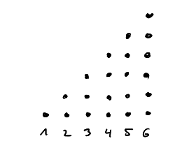
We visualize the number \(i\) simply as a set of \(i\) points. For convenience we place all these points in one column. Taking the sum now simply means taking the disjoint union of these sets of points. In case of the sum \(\sum_{i=1}^n i\) this yields a triangle of points.

Now, we have no idea (yet) how to count point in triangles. But we have a very good idea of how to count points in rectangles: that’s just what multiplication is for! So we take two instances of this triangle and fit them together such that they form a rectangle of \(n\) by \(n+1\) points.

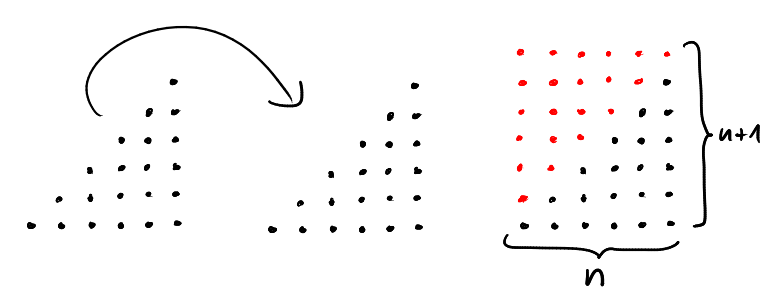
This shows \[2\cdot \sum_{i=1}^n i = n(n+1)\] which implies Gauss’ formula.

Note: A video in which I tell just this story in German can be found here.

Lattice Points in Triangles

Crucial to the above argument was that we arranged the points in a regular pattern. In fact, we used points \(x\) in the lattice \(\mathbb{Z}^2\). Throughout these lectures a lattice point or integer point will be an element of the integer lattice \(\mathbb{Z}^n\) for some \(n\). There are other lattices, but we will only work with this one. For convenience, we will write \(L(X)= |\mathbb{Z}^n\cap X|\) for the number of lattice points in some set \(X\subset\mathbb{R}^n\).

In the above proof, we used the set of lattice points contained in the triangle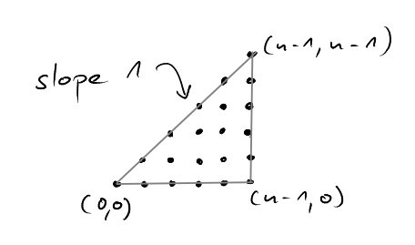

The two "instances" of this triangle fit together so nicely, because the line \(x_1=x_2\) corresponding to the inequality \(x_1\geq x_2\) has slope 1. Thus, whenever we move one column to the right, the number of lattice points in the column always changes by one. What happens when we consider triangles with more general (rational) slopes?

Let \(T_{a,b}\) denote the triangle with slope \(\frac{b}{a}\) for \(a,b\in\mathbb{N}\).

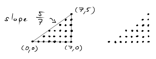
Here, the "steps" we take from one column to the next become irregular. Sometimes we go one lattice point up, sometimes we don’t. But before we take another look at the structure of this lattice point set, let us simply count how many lattice points there are.

Counting Lattice Points

Counting the number of lattice points in \(T_{a,b}\) is easy enough.

\[ L(T_{a,b}) = |\mathbb{Z}^2 \cap T_{a,b}| = \sum_{k=0}^a \left( \left\lfloor \frac{kb}{a} \right\rfloor + 1 \right)\]

But what we really want is a simple expression for the sum on the right hand side. Let us try a variation of the previous trick to find one!

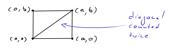We can fit two "instances" of the triangle \(T_{a,b}\) together to form the rectangle \(R=[0,a]\times[0,b]\). All lattice points in \(R\) are contained in exactly one of the two triangles, except for the lattice points on the diagonal

The lattice points on the diagonal \(D\) are contained in both triangles and are thus counted twice in the following sum.

So how many lattice points are on the diagonal?

Lemma. The number of lattice points on the diagonal \(D_{a,b}\) is the greatest common divisor of \(a\) and \(b\) plus one, that is, \[L(D_{a,b}) = \text{gcd}(a,b) +1.\]

Proof. We make the following observations.

1. The lattice points on the diagonal parition the diagonal into intervals of equal length.

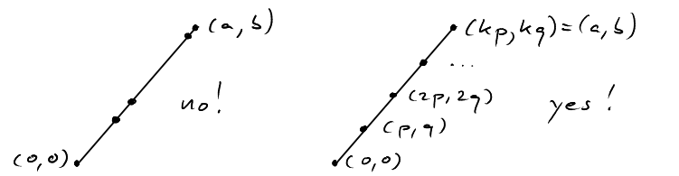
This follows simply from the fact that the difference between to lattice points is an integer vector and translation by an integer vector maps lattice points to lattice points.

2. Let \((p,q)\in D\cap\mathbb{Z}^2\) such that \(p>0\) is minimal. Let \(k\) be the number of intervals into which \(D\) is partitioned. Then \[kp = a \;\;\; \text{and} \;\;\; kq = b.\] So \(k\) is a common divisor of \(a\) and \(b\).

3. Conversely, let \(k'\) be a common divisor of \(a\) and \(b\). This means, there exist \(p',q'\in \mathbb{Z}^2\) such that \[ k'p' = a \;\;\; \text{and} \;\;\; k'q' = b,\] which implies \(\begin{pmatrix} p \\ q\end{pmatrix}=\frac{1}{k'}\begin{pmatrix} a \\ b\end{pmatrix},\) which in turn means that \((p',q')\) is a lattice point on the diagonal \(D_{a,b}\).

As \(p\) was chosen minimal, we conclude that \(p' \geq p\) and thus \(k' \leq k\), which means that \(k\) is the greatest common divisor of \(a\) and \(b\). The number of lattice points on the diagonal is \(k+1\). QED.

Great! Now we have both: a visual interpretation of the \(\text{gcd}\) and the means to complete our formula!

\[\sum_{k=0}^a \left( \left\lfloor \frac{kb}{a} \right\rfloor + 1 \right) = \frac{(a+1)(b+1) + \text{gcd}(a,b) + 1}{2}\]

Note that by symmetry we also get

\[\sum_{k=0}^b \left( \left\lfloor \frac{ka}{b} \right\rfloor + 1 \right) = \frac{(a+1)(b+1) + \text{gcd}(a,b) + 1}{2}.\]

This corresponds to the fact that the lattice point sets in \(T_{a,b}\) and \(T_{b,a}\) are "the same". Let us make this notion precise.

Lattice Isomorphism

We want to answer questions such as "How many lattice points are in a set \(S\)?" From this point of view, we want to see two sets as "the same" when there is a linear automorphism from the ambient space to itself that induces a bijection on the lattice. Then, applying the automorphism does not changes the number of lattice points in any given set.

So, a lattice isomorphism is an affine linear map \(f:\mathbb{R}^n\rightarrow\mathbb{R}^n\) of the form \(f(x)=Ax+b\) that induces a bijection from \(\mathbb{Z}^n\) onto itself. We say set \(X\) is a lattice transform of a set \(Y\) if there exists a lattice isomorphism \(f\) with \(f(X)=Y\).

Lattice isomorphisms are very useful objects. We have already made implicit use of the fact that translations by an integer vector and reflections at the origin are lattice isomorphisms. And our observation that \(T_{a,b}\) and \(T_{b,a}\) have "the same" lattice point structure can be made precise by saying that

is a lattice isomorphism.

We will need one more lattice isomorphism in a minute. And to show that it is a lattice isomorphism, we will make use of the following tool.

Lemma. The map \(x\mapsto Ax +b\) is a lattice isomorphism if and only if \(A\) and \(b\) are integral and \(\det(A) = \pm 1\).

The proof is not difficult, and we omit it for now.

Structure of \(\mathbb{Z}^2\cap T_{a,b}\)

We now know how many lattice points there are in \(T_{a,b}\). But what we would really like to understand is the structure of this set of lattice point. When we look at larger examples of these triangles than we see that this "staircase" of points appears "irregular" but far from "random". What is going on here?

One way to approach this question is by investigating the recursive structure of these lattice point sets. We can ask:

What subset of \(\mathbb{Z}^2\cap T_{a,b}\) is particularly easy to describe?

As we have seen in the example of Gauss’ sum formula, triangles with integral slopes are particularly easy to describe.

Let us suppose that \(a < b\). This means that the slope \(\frac{b}{a}\) of the triangle is "steep". In this case, we can find a subset of the lattice points which corresponds to a triangle with integral slope. Or, more precisely, \[\mathbb{Z}^2\cap T_{a,a} \subset \mathbb{Z}^2\cap T_{a,b}.\]

Let us split the triangle \(T_{a,b}\) into two parts. A lower part with integral slope that is easy to describe and an upper part that we have yet to make sense of. Both parts meet at the line \(x_1=x_2\). For convenience, we decide that this boundary should belong to the upper part and it should be removed from the lower part. The lower part then becomes a half-open triangle of the form

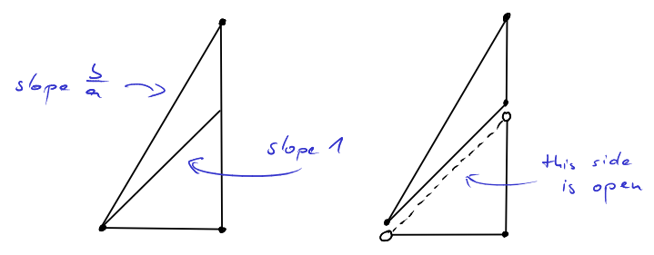
In this way we can partition \(T_{a,b}\) such that

the lower part \(\mathbb{Z}^2\cap T'_{a,a}\) has a simple form and precisely \(\frac{a(a+1)}{2}\) lattice points.

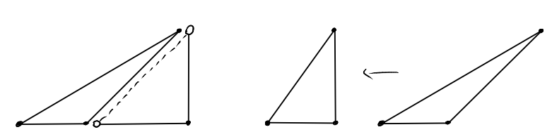
Good. What about the upper part \(T_{a,b}\setminus T'_{a,a}\)?

We would like to see that this upper part is again a triangle of the form we have been studying all the time, so that we apply recursion. To that end we need to transform the upper part so as to create a right angle at the vertex on the bottom-right. To achieve this we might try to shear the triangle. But is the resulting linear transformation a lattice isomorphism?

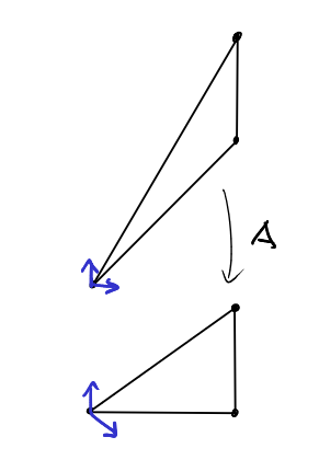As we can see the matrix of the linear transformation is simply

As \(\det(A)=1\) we conclude that this transformation is a lattice isomorphism and thus:

The upper part \(T_{a,b}\setminus T'_{a,a}\) is a lattice transform of \(T_{a,b-a}\).

So we can simplify "steep" triangles until we obtain a "flat" triangle with slope \(<1\). But by our observation that

\(T_{a,b}\) is a lattice transform of \(T_{b,a}\)

we can turn "flat" triangles into "steep" triangles and continue with this method of simplification! Equivalently, we can handle flat triangles by partitioning them differently and shearing "left" instead of "down".

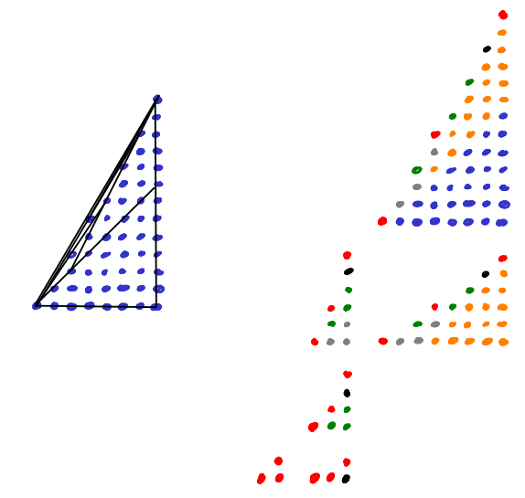
We have thus obtained a recursive description of the sets of lattice points in the triangles \(T_{a,b}\).

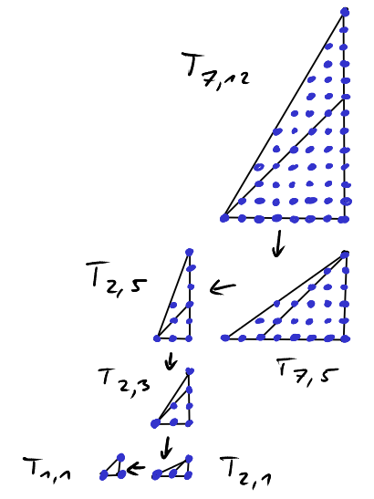
This allows us to decompose the set of lattice points in a large triangle \(T_{a,b}\) into lattice transforms of "simple" sets of lattice points.

(Note: There are other ways of making sense of this "staircase" of lattice points. If you got curious, I would like to advertise Fred’s and my article on "Staircases in \(\mathbb{Z}^2\)".)

As a side-effect, this recursion also allows us to count the lattice points in \(T_{a,b}\) recursively.

Theorem. Let \(a,b\in\mathbb{N}\). Then:

1. If \(a>b\) then \(L(T_{a,b})=L(T_{a-b,b}) + \frac{b(b+1)}{2}\).
2. If \(a < b\) then \(L(T_{a,b})=L(T_{a,b-a}) + \frac{a(a+1)}{2}\).
3. \(L(T_{a,a})=\frac{(a+1)(a+2)}{2}\).

Apart from the structural insight, what does the recursion for \(L(T_{a,b})\) buy us? With \[L(T_{a,b})=\frac{(a+1)(b+1) + \text{gcd}(a,b) + 1}{2}\] we already have a very nice closed form expression for \(L(T_{a,b})\), don’t we?

Well, not quite. \(\text{gcd}(a,b)\) is no closed form expression. To compute \(\text{gcd}(a,b)\) we need to use the Euclidean Algorithm. In fact, I would like to argue that the above recursion is essentially the same as the Euclidean Algorithm.

Visualizing the Euclidean Algorithm

I would like to close this lecture by arguing that the recursion we developed in the previous section is nothing but a visualization of the Euclidean Algorithm. A simple description of the Euclidean Algorithm (which he called "antenaresis") is this:

"[The greatest common divisor] can be found using antenaresis by repeatedly subtracting the smaller, whichever it happens to be at the time, from the larger until the smaller divides the larger." Euclid’s Elements

When we apply the above recursion to compute \(L(T_{a,b})\), we do exactly the same thing, as far as the pair \((a,b)\) is concerned! If \(a>b\) we pass to \((a-b,b)\) and if \(a < b\) we pass to \((a,b-a)\). Even the stopping criteria are essentially the same, even though they look different at first glance.

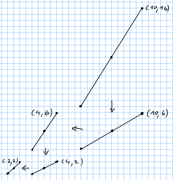
So here is a "geometric interpretation" of the Euclidean Algorithm:

1. We want to compute the greatest common divisor of \(a\) and \(b\). As we have seen this amounts to computing the number of lattice points on the diagonal \(D_{a,b}\) of the rectangle \([0,a]\times[0,b]\).
2. To achieve this, we apply lattice transformations. These do not change the number of lattice points on the diagonal.

• If \(a > b\) we shear the diagonal "left" and pass to \(D_{a-b,b}\).
• If \(a < b\) we shear the diagonal "down" and pass to \(D_{a,b-a}\).

3. We stop as soon as the number of lattice points on the diagonal can be read of immediately. For example, if we reach a line of the form \(D_{a,a}\) or \(D_{a,ka}\) or \(D_{a,0}\).

So in a way,

all the Euclidean Algorithm does is compressing a set of lattice points by means of lattice transformations!

For our two formulas for \(L(T_{a,b})\) this means that both use the same type of recursion. This of course begs the question:

Is there a faster way to compute the \(\text{gcd}\) of two integers? Is there maybe even a "closed form" expression for \(\text{gcd}\)?

As it turns out, these questions are closely related to a long standing open problem in complexity theory:

Is the problem of computing the \(\text{gcd}\) in the complexity class \(\mathbf{AC}\)?

Informally, this is asking whether there exists a family of boolean circuits with polynomial size, polylogarithmic-depth and unbounded fan-in that computes the \(\text{gcd}\). See the Complexity Zoo for more information.

Outlook

This is it for today! Next time, we will continue visualizing numbers and venture into the world of Dedekind sums.