There are many beautiful geometric interpretations of the GCD and visualizations of the Euclidean algorithm out there, see for example here, here and here. I have written about this myself some time ago. But I find that some of the pictures become much clearer when lifted into the third dimension.

[Note: I am using Sage Cells to produce the pictures in this post. This has the advantage that you, dear reader, can interact with the pictures by modifying the Sage code. However, this will probably not run everywhere. It certainly won’t work in most RSS readers…]

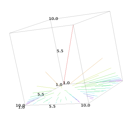
Here is the graph of the GCD! First a little static preview…

… and now a proper interactive graph. Be sure to rotate the image to get a 3d impression. (Requires Java…)

What precisely are we seeing here? The gcd is a function $\mathrm{gcd}:\mathbb{N}^2\rightarrow\mathbb{N}$. Its graph is a (countable) set of points in $\mathbb{N}^3$. This graph is precisely the set of integer points contained in one of the (countably many) lines indicated in the above picture. The value of the gcd is given by the vertical axis.

Now, what are those lines? Suppose $a$ and $b$ are two natural numbers that are relatively prime, i.e., $\gcd(a,b)=1$. Then we know that $\gcd(ka,kb)=k$ for any positive integer $k$. So all (positive) integer points on the line through the origin and $(a,b,1)$ are in the graph of the gcd. Conversely, for any numbers $x,y$ with $gcd(x,y)=z$, we know that $\gcd(\frac{x}{z},\frac{y}{z})=1$, that is, the point $(x,y,z)$ lies on the line through the origin and $(\frac{x}{z},\frac{y}{z},1)$. So by drawing all these lines, we can be sure we hit all the integer points in the graph of the gcd.

What I find very beautiful about this is that when looking at this picture from the right angle, you can see the binary tree structure of this set of lines. It is precisely this binary tree that we walk along when running the Euclidean algorithm. The lines in the above picture are color coded by their depth in this “Euclidean” binary tree.

The version of the Euclidean algorithm I like best this one. Suppose you want to find $\gcd(a,b)=1$. If $a>b$, compute $\gcd(a-b,b)$. If $a<b$, compute $\gcd(a,b-a)$. If $a=b$, we are done and the number $a=b$ is the gcd. At each point in the algorithm we make a choice, depending on whether $a>b$ or $a<b$. If we keep track of these choices by writing down a 1 in the former case and a 0 in the latter, then, for any pair (a,b), we get a word of 0s and 1s that describes a path through a binary tree. As we walk from one pair $(a,b)$ to the next in this fashion, we trace out a path in the plane: For each 1 we take a horizontal step and for each 0 we take a vertical step. This path can look as follows.

Now comes the twist. We can turn the Euclidean algorithm upside down. Instead of walking from the point $(a,b)$ to a point of the form $(g,g)$ and thus finding the gcd, we can also start from the point $(1,1)$ and walk to a point of the form $(\frac{a}{g},\frac{b}{g})$ to find the gcd $g$. (Why $(\frac{a}{g},\frac{b}{g})$? Well, $(\frac{a}{g},\frac{b}{g})$ is the primitive lattice vector in the direction of $(a,b)$. In terms of the graph at the top, $(\frac{a}{g},\frac{b}{g},1)$ is the starting point of the ray through $(a,b,\gcd(a,b))$.)

How do we get there? We start out by fixing the lattice basis with “left” basis vector $(0,1)$ and “right” basis vector $(1,0)$. Their sum $(1,1)$, which I call the “center”, is a primitive lattice vector. Now we ask ourselves: is the point $(a,b)$ to the left or to the right of the line through the center? If it is to the left of that line, we continue with the basis $(0,1)$ and $(1,1)$. If it is to the right of that line, we continue with the basis $(1,1)$ and $(1,0)$ and recurse: We take the sum of our two new basis vectors as the new center and ask if $(a,b)$ lies to the left or to the right of the line through the center, and continue accordingly. If $(a,b)$ lies on the line through the center, we are done: the gcd of $a$ and $b$ is the factor by which I have to multiply the center to get to $(a,b)$.

As we follow this algorithm, we draw the path from one center to the next, until we reach $(\frac{a}{g},\frac{b}{g})$. Then we get the following picture. It looks almost like a straight line from $(1,1)$ to our goal, but it is only straight whenever we take two consecutive left turns or two consecutive right turns. Whenever we alternate between right and left, we have a proper angle, it only gets difficult to see this angle the farther out we get. If we write down a sequence of 1s and 0s, corresponding to the left and right turns we take, we get the exact same sequence as with the standard Euclidean algorithm.

The obvious next step is to draw the complete binary trees given by the above two visualizations of the Euclidean algorithm (up to a certain maximum depth). Drawing the first tree gives a big mess, because many of the edges of the tree overlap. You can clean up the picture by removing the lines and drawing only the points: In the code below comment the first definition of thisdrawing and uncomment the second. This then gives you a picture of all primitive lattice points (pairs of relatively prime numbers) in the plane at depth at most maxdepth in the tree.

The second variant of the Euclidean algorithm gives a much nicer picture, revealing the fractal nature of the set of primitive lattice points. The nodes of the tree, i.e., the points drawn in the picture are the starting points of the rays plotted in the 3d graph of the gcd given at the beginning of this post. In this way, this drawing of the tree gives the precise structure of the binary tree intuitively visible in the three-dimensional graph. One thing you may want to try is to increase the maxdepth of the tree to 10. (Warning: this may take much longer to render!) Note how far out from the origin some of the points at depths 10 are.

The reader may have observed that the binary tree described in this post gives us a very nice way of enumerating the rational numbers. Calkin and Wilf made this observation in the paper Recounting the Rationals, whence it is sometimes called the Calkin-Wilf tree, even though Euclid tree might be a better name as it is given by the Euclidean algorithm itself. As we have seen above, a look through the lens of lattice geometry tells us how to draw this tree in the plane and how to find it in the graph of the GCD.